Parameterization vs Performance
Best ROC and PRC
In this section we will compare the normalized combined predictors (\(calibrated + \beta \times random, \beta=-1\)) across all 3 model parameterizations/mutations we tested in this report for CASCADE 2.0: link operator mutations, topology mutations and both. We use the normalization parameter \(\beta=-1\) for all combined predictors, as it was observed throughout the report that it approximately maximizes the performance of all Bliss-assessed, ensemble-wise combined synergy predictors in terms of ROC and PR AUC. The results are from the \(150\) simulation runs (\(450\) models).
Why call \(\beta\) a normalization parameter?
What matters for the calculation of the ROC and PR points is the ranking of the synergy scores. Thus if we bring the predictor’s synergy scores to the exponential space, a value of \(-1\) for \(\beta\) translates to a simple fold-change normalization technique:
\(calibrated + \beta \times random \overset{\beta = -1}{=} calibrated - random \xrightarrow[\text{same ranking}]{e(x) \text{ monotonous}}\) \(e^{(calibrated - random)}=e^{calibrated}/e^{random}\).
# Link operator mutations results (`best_score2` has the results for β = -1, `best_score1` for β = -1.6)
roc_link_res = get_roc_stats(df = pred_ew_bliss, pred_col = "best_score2", label_col = "observed")
pr_link_res = pr.curve(scores.class0 = pred_ew_bliss %>% pull(best_score2) %>% (function(x) {-x}),
    weights.class0 = pred_ew_bliss %>% pull(observed), curve = TRUE, rand.compute = TRUE)

# Topology mutations results
roc_topo_res = get_roc_stats(df = pred_topo_ew_bliss, pred_col = "best_score", label_col = "observed")
pr_topo_res = pr.curve(scores.class0 = pred_topo_ew_bliss %>% pull(best_score) %>% (function(x) {-x}),
    weights.class0 = pred_topo_ew_bliss %>% pull(observed), curve = TRUE)

# Both Link Operator and Topology mutations results
roc_topolink_res = get_roc_stats(df = pred_topolink_ew_bliss, pred_col = "best_score", label_col = "observed")
pr_topolink_res = pr.curve(scores.class0 = pred_topolink_ew_bliss %>% pull(best_score) %>% (function(x) {-x}),
    weights.class0 = pred_topolink_ew_bliss %>% pull(observed), curve = TRUE)

# Plot best ROCs
plot(x = roc_link_res$roc_stats$FPR, y = roc_link_res$roc_stats$TPR,
  type = 'l', lwd = 3, col = my_palette[1], main = TeX('ROC curves (Ensemble-wise), $calibrated + \\beta \\times random$'),
  xlab = 'False Positive Rate (FPR)', ylab = 'True Positive Rate (TPR)')
lines(x = roc_topo_res$roc_stats$FPR, y = roc_topo_res$roc_stats$TPR,
  lwd = 2, col = my_palette[2])
lines(x = roc_topolink_res$roc_stats$FPR, y = roc_topolink_res$roc_stats$TPR,
  lwd = 2.3, col = my_palette[3])
legend('bottomright', title = TeX('AUC ($\\beta$ = -1): Mutations'),
  col = c(my_palette[1:3]), pch = 19, cex = 1.5,
  legend = c(paste(round(roc_link_res$AUC, digits = 2), 'Link Operator'),
    paste(round(roc_topo_res$AUC, digits = 2), 'Topology'),
    paste(round(roc_topolink_res$AUC, digits = 2), 'Both')))
grid(lwd = 0.5)
abline(a = 0, b = 1, col = 'lightgrey', lty = 'dotdash', lwd = 1.2)

# Plot best PRCs
plot(pr_link_res, main = TeX('PR curves (Ensemble-wise), $calibrated + \\beta \\times random$'),
  auc.main = FALSE, color = my_palette[1], rand.plot = TRUE, lwd = 3)
plot(pr_topo_res, add = TRUE, color = my_palette[2], lwd = 2)
plot(pr_topolink_res, add = TRUE, color = my_palette[3], lwd = 2.3)
legend('topright', title = TeX('AUC ($\\beta$ = -1): Mutations'),
  col = c(my_palette[1:3]), pch = 19, cex = 1.3,
  legend = c(paste(round(pr_link_res$auc.davis.goadrich, digits = 2), 'Link Operator'),
    paste(round(pr_topo_res$auc.davis.goadrich, digits = 2), 'Topology'),
    paste(round(pr_topolink_res$auc.davis.goadrich, digits = 2), '  Both')))
grid(lwd = 0.5)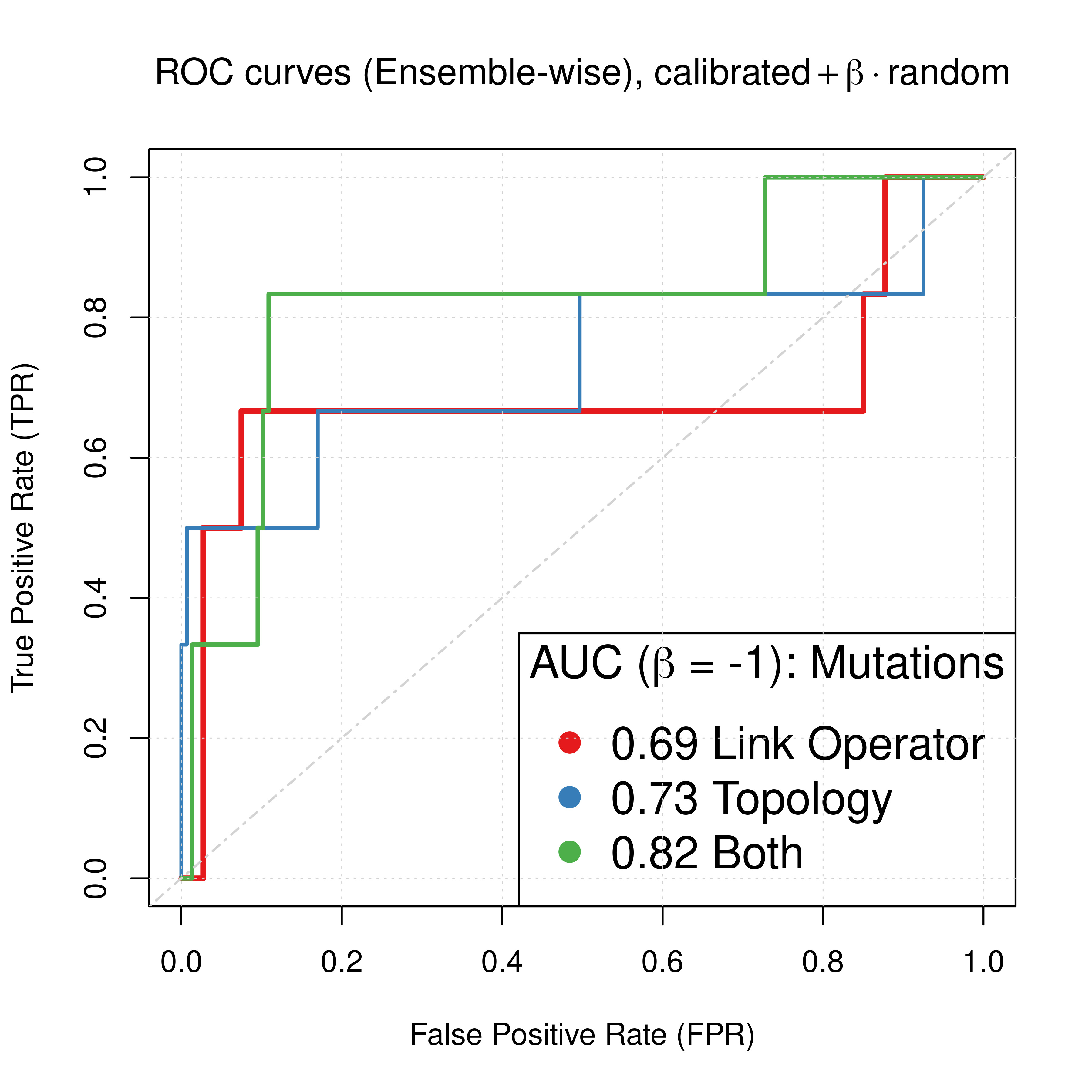
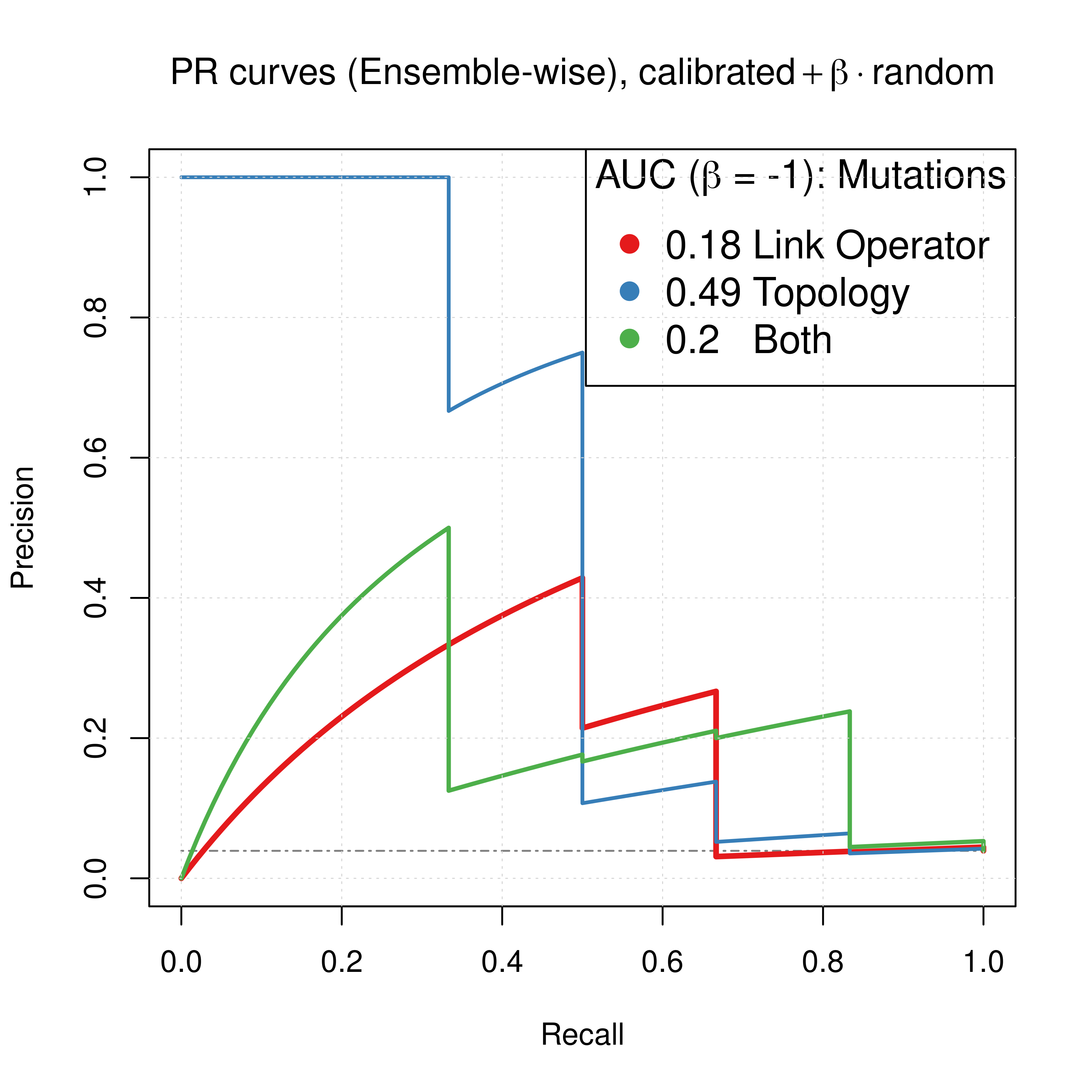
Figure 65: Comparing ROC and PR curves for combined predictors across 3 parameterization schemes (CASCADE 2.0, Bliss synergy method, Ensemble-wise results)
We observe that if we had used the results for the link operator only combined predictor with \(\beta_{best}=-1.6\) as was demonstrated here, we would have an AUC-ROC of \(0.85\) and AUC-PR of \(0.27\), which are pretty close to the results we see above for \(\beta=-1\), using both link and topology mutations.
Overall, this suggests that to parameterize our boolean models using topology mutations can increase the performance of our proposed synergy prediction approach much more than using either link operator (balance) mutations alone or combined with topology parameterization.
Note that the difference in terms of ROC AUC is not significant compared to the difference of PR AUC scores and since the dataset we test our models on is fairly imbalanced, we base our conclusion on the information from the PR plots (Saito and Rehmsmeier 2015).
Bootstrap Simulations
Now we would like to statistically verify the previous conclusion (that topology is superior to the other two parameterization schemes and produces better predictive models for our dataset) and so we will run a bootstrap analysis.
Simply put, we generate 3 large pools of calibrated to steady state models (\(4500\) models each). Each pool corresponds to the 3 parameterization schemes (i.e. it has models with either topology mutations only, link-operator mutations only, or models with both mutations). Then, we take several model samples from each pool (\(25\) samples, each sample containing \(300\) models) and run the drug response simulations for these calibrated model ensembles to get their predictions. Normalizing each calibrated simulation prediction output to the corresponding random (proliferative) model predictions (using a \(\beta=-1\) as above), results in different ROC and PR AUCs for each parameterization scheme and chosen bootstrapped sample.
See more details on reproducing the results on section Parameterization Bootstrap.
Load the already-stored result:
res = readRDS(file = "data/res_param_boot_aucs.rds")Compare all 3 schemes
# define group comparisons for statistics
my_comparisons = list(c("link-only","topology-only"), c("link-only","topo-and-link"),
  c("topology-only","topo-and-link"))

# ROC AUCs
ggboxplot(data = res, x = "param", y = "roc_auc",
  fill = "param", add = "jitter", palette = "Set1",
  xlab = "Parameterization", ylab = "ROC AUC",
  title = "Parameterization vs Performance (ROC)") +
  stat_compare_means(comparisons = my_comparisons, method = "wilcox.test", label = "p.format") +
  theme(plot.title = element_text(hjust = 0.5)) +
  theme(legend.position = "none")

# PR AUCs
ggboxplot(data = res, x = "param", y = "pr_auc",
  fill = "param", add = "jitter", palette = "Set1",
  xlab = "Parameterization", ylab = "PR AUC",
  title = "Parameterization vs Performance (Precision-Recall)") +
  stat_compare_means(comparisons = my_comparisons, method = "wilcox.test", label = "p.format") +
  theme(plot.title = element_text(hjust = 0.5)) +
  theme(legend.position = "none")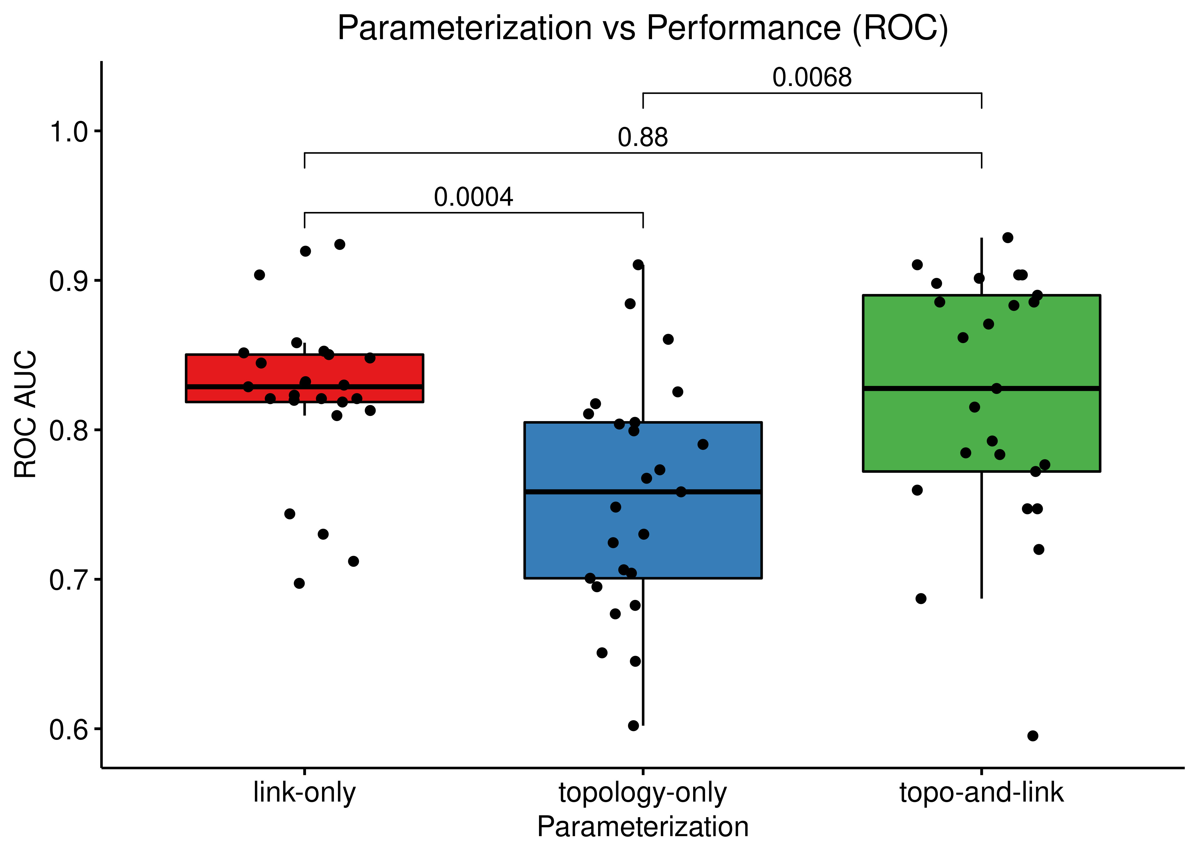
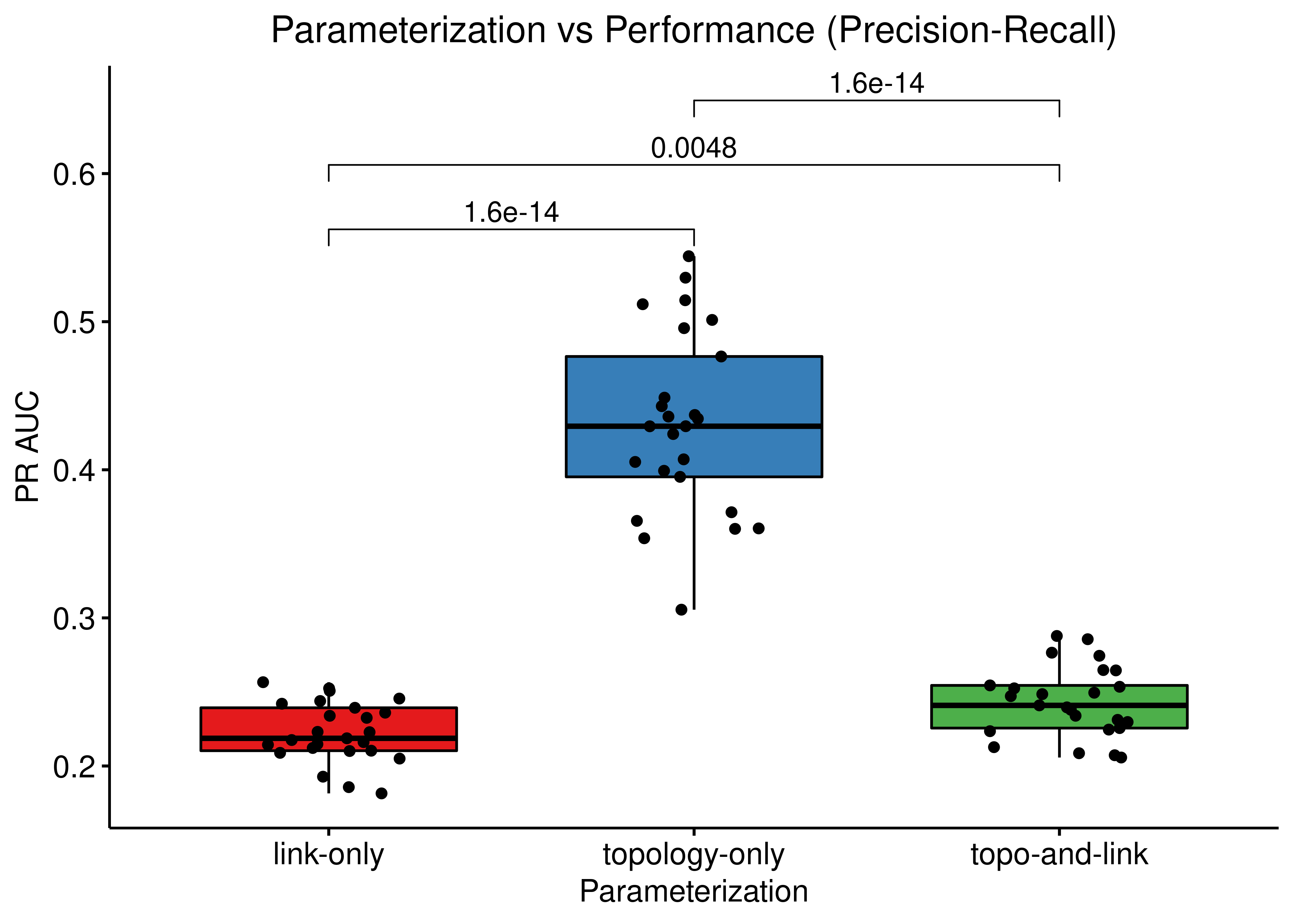
Figure 66: Comparing ROC and PR AUCs from bootstrapped calibrated model ensembles normalized to random model predictions across 3 parameterization schemes (CASCADE 2.0, Bliss synergy method, Ensemble-wise results)
The topology mutations generate the best performing models in terms of PR AUC with statistical significance compared to the other two groups of model ensembles using different parameterization. In terms of ROC AUC performance we also note the larger variance of the topology mutated models.
Compare Topology vs Link-operator Parameterization
# load the data
res = readRDS(file = "data/res_param_boot_aucs.rds")

# filter data
res = res %>%
  filter(param != "topo-and-link")

param_comp = list(c("link-only","topology-only"))

stat_test_roc = res %>%
  rstatix::wilcox_test(formula = roc_auc ~ param, comparisons = param_comp) %>%
  rstatix::add_significance("p")

# ROC AUCs
ggboxplot(res, x = "param", y = "roc_auc", fill = "param", palette = "Set1",
  add = "jitter", xlab = "", ylab = "ROC AUC") +
  scale_x_discrete(breaks = c("link-only","topology-only"),
    labels = c("Parameterization Mutations", "Topology Mutations")) +
  ggpubr::stat_pvalue_manual(stat_test_roc, label = "p = {p} ({p.signif})", y.position = c(1)) +
  ylim(c(0.2,1)) +
  theme_classic(base_size = 14) +
  theme(plot.title = element_text(hjust = 0.5), axis.text = element_text(size = 16)) +
  geom_hline(yintercept = 0.5, linetype = 'dashed', color = "red") +
  geom_text(aes(x = 2.1, y = 0.45, label="Random Predictions (AUC = 0.5)", size = 5)) +
  theme(legend.position = "none")

stat_test_pr = res %>%
  rstatix::wilcox_test(formula = pr_auc ~ param, comparisons = param_comp) %>%
  rstatix::add_significance("p") %>%
  rstatix::add_y_position()

# PR AUCs
ggboxplot(res, x = "param", y = "pr_auc", fill = "param", palette = "Set1",
  add = "jitter", xlab = "", ylab = "Precision-Recall AUC") +
  scale_x_discrete(breaks = c("link-only","topology-only"),
    labels = c("Parameterization Mutations", "Topology Mutations")) +
  ggpubr::stat_pvalue_manual(stat_test_pr, label = "p = {p} ({p.signif})") +
  theme_classic(base_size = 14) +
  theme(plot.title = element_text(hjust = 0.5), axis.text = element_text(size = 16)) +
  geom_hline(yintercept = 6/153, linetype = 'dashed', color = "red") +
  geom_text(aes(x = 1.9, y = 0.08, label="Random Predictions (AUC = 0.04)"), size = 5) +
  theme(legend.position = "none")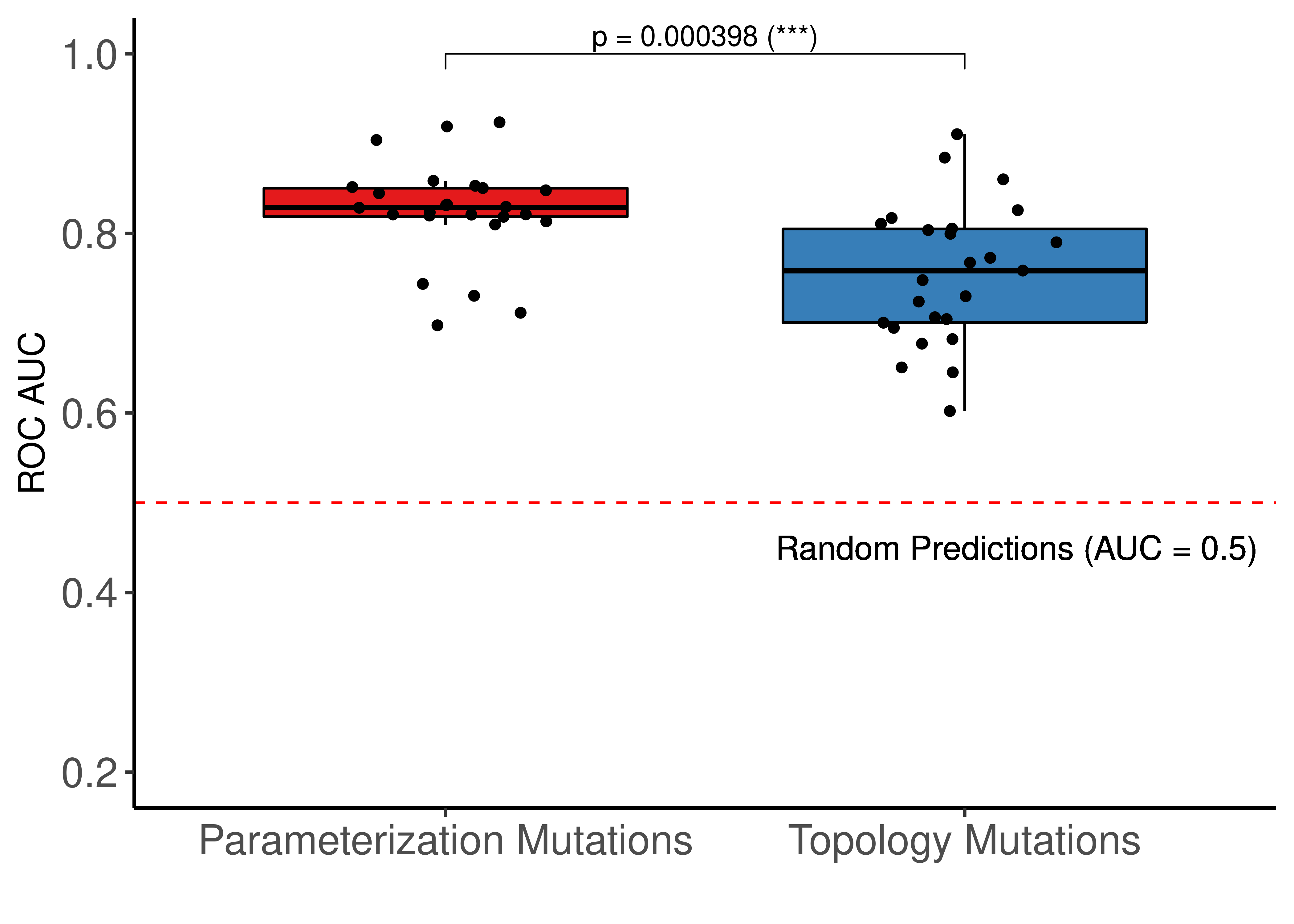
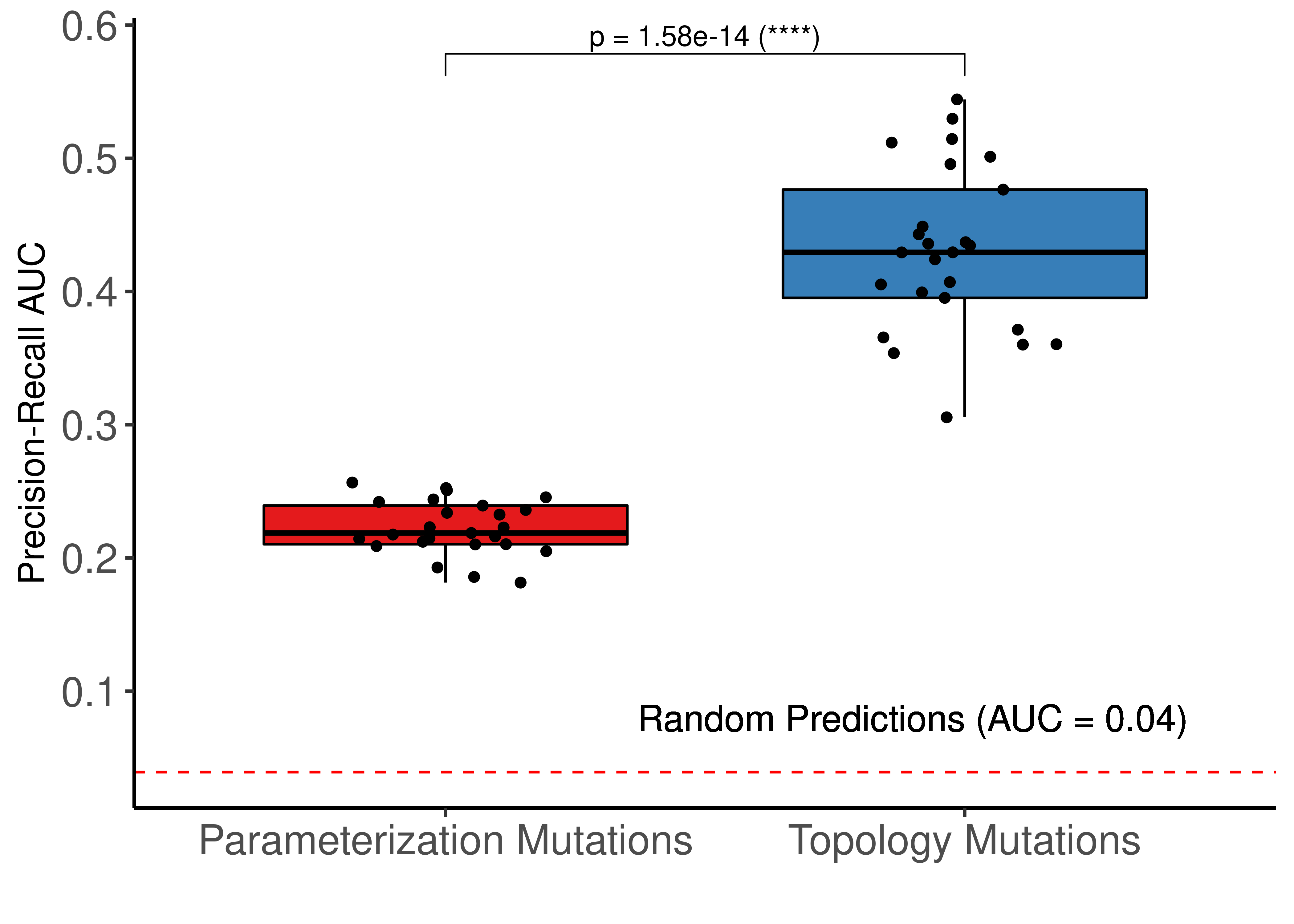
Figure 67: Comparing ROC and PR AUCs from bootstrapped calibrated model ensembles normalized to random model predictions - Topology vs Link-operator mutations (CASCADE 2.0, Bliss synergy method, Ensemble-wise results). We use the terminology “parameterization” to refer to the link operator mutations