Mouse Xenograft Results
Figures for the paper from the mouse experiments. Mice were injected with AGS tumors and split to \(4\) groups:
Controlgroup (no drugs were administered)- Mice group which was administered a TAK1 inhibitor (
5Zdrug) - Mice group which was administered a PI3K inhibitor (
PIdrug) - Mice group which was administered both
5ZandPIdrugs
# read file with tumor volume data
tumor_data = readr::read_csv(file = 'data/tumor_vol_data.csv')
tumor_data_wide = tumor_data # keep the wide format for later

# reshape data
tumor_data = tumor_data %>%
  tidyr::pivot_longer(cols = -c(drugs), names_to = 'day', values_to = 'vol') %>%
  mutate(day = as.integer(day)) %>%
  mutate(drugs = factor(x = drugs, levels = c("PI", "Control", "5Z", "5Z-PI")))
pd = position_dodge(0.2)
days = tumor_data %>% distinct(day) %>% pull()
tumor_data %>%
ggpubr::desc_statby(measure.var = 'vol', grps = c('day', 'drugs')) %>%
ggplot(aes(x = day, y = mean, colour = drugs, group = drugs)) +
geom_errorbar(aes(ymin = mean - se, ymax = mean + se), color = 'black',
width = 1, position = pd) +
geom_line(position = pd) +
geom_point(position = pd) +
scale_x_continuous(labels = as.character(days), breaks = days) +
scale_color_brewer(palette = 'Set1') +
labs(title = 'Average tumor volume with SEM', x = 'Days',
y = latex2exp::TeX('Tumor volume $\\left(mm^3\\right)$')) +
ylim(c(0, NA)) +
theme_classic(base_size = 14) +
theme(plot.title = element_text(hjust = 0.5), legend.title = element_blank())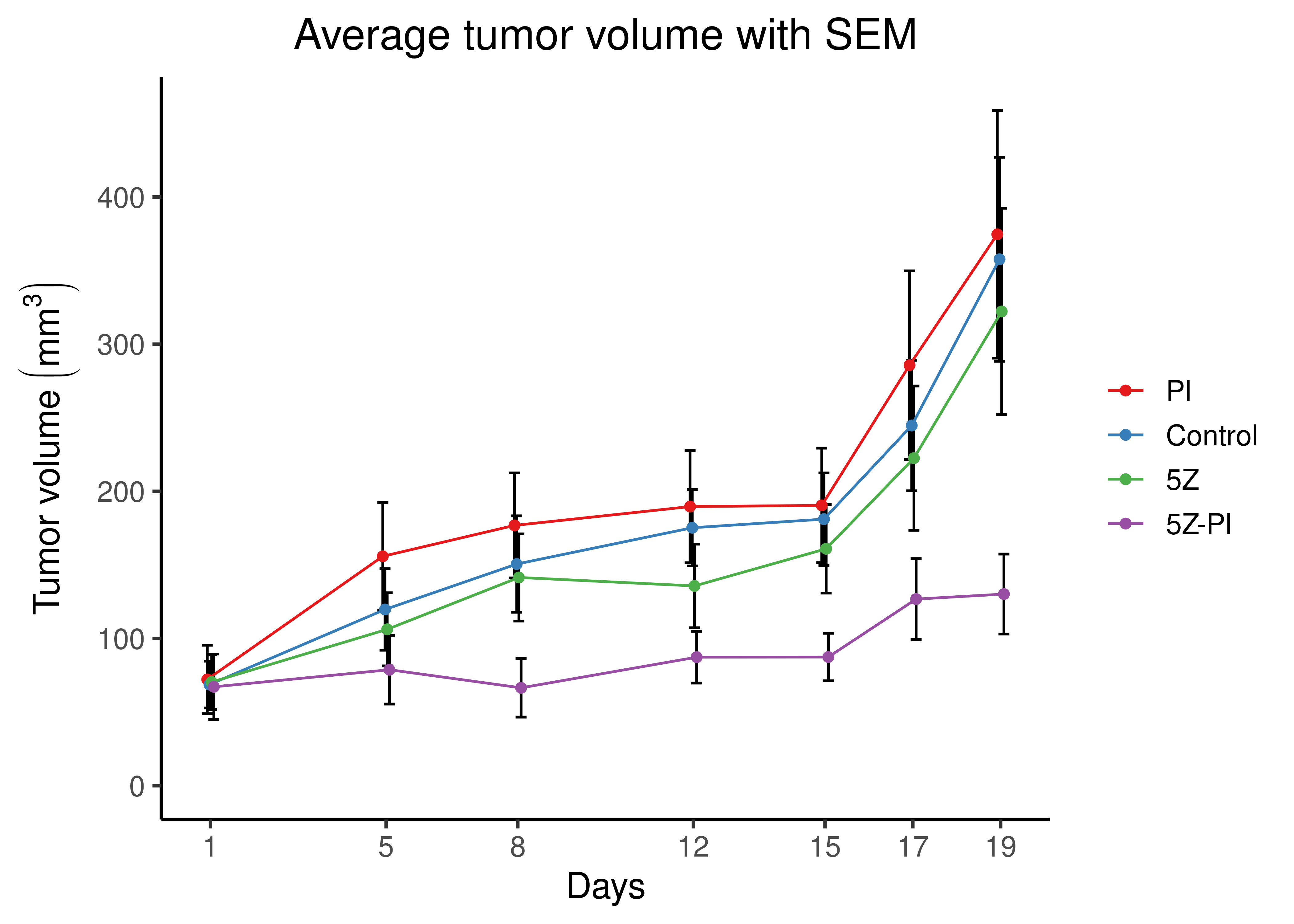
Figure 78: Average tumor volume and standard error of the mean (SEM) for the four groups of mice, per measurement day after tumor injection (1st day)
We use the Wilcoxon rank sum test to compare the tumor values between the different mice groups (adjusted p-values are calculated using Holm’s method (Holm 1979; Aickin and Gensler 1996):
tumor_wilcox_res = tumor_data %>%
  rstatix::wilcox_test(formula = vol ~ drugs)%>% select(-`.y.`)

DT::datatable(data = tumor_wilcox_res, options = list(pageLength = 6)) %>%
  DT::formatStyle('p.adj', backgroundColor = 'lightgreen')
We also demonstrate the mouse survival plots and compute a p-value using the log-rank non-parametric test, which shows that the survival curves are not identical.
We chose the median tumor value of the PZ-PI mice group on day \(19\) as the threshold to define the status indicator (\(0=\text{alive}, 1=\text{death}\)) for each mouse measurement and compute the survival probabilities using the Kaplan-Meier method.
# specify a tumor volume value, less than which, signifies that the tumor
# is "dead" or equivalently, that the mouse "survives"
tumor_thres = tumor_data %>%
  filter(day == 19, drugs == "5Z-PI") %>%
  summarise(med = median(vol)) %>%
  pull()

# for coloring
set1_col = RColorBrewer::brewer.pal(n = 4, name = 'Set1')

# 0 = alive, 1 = dead mouse!
td = tumor_data %>% mutate(status = ifelse(vol < tumor_thres, 0, 1))
fit = survival::survfit(survival::Surv(day, status) ~ drugs, data = td)
survminer::ggsurvplot(fit, palette = set1_col[c(2,1,3,4)],
  fun = "pct", xlab = "Days", ylab = "Event Probability (%)",
  pval = TRUE, pval.method = TRUE, surv.median.line = "hv",
  pval.size = 8, pval.coord = c(2,25),  pval.method.coord = c(2,15),
  #risk.table = TRUE,
  # confidence intervals don't look good because of small number of days
  #conf.int = TRUE, conf.int.style = "ribbon", conf.int.alpha = 0.5,
  break.x.by = 2,
  legend.labs = c("Control", "PI", "5Z", "5Z-PI"))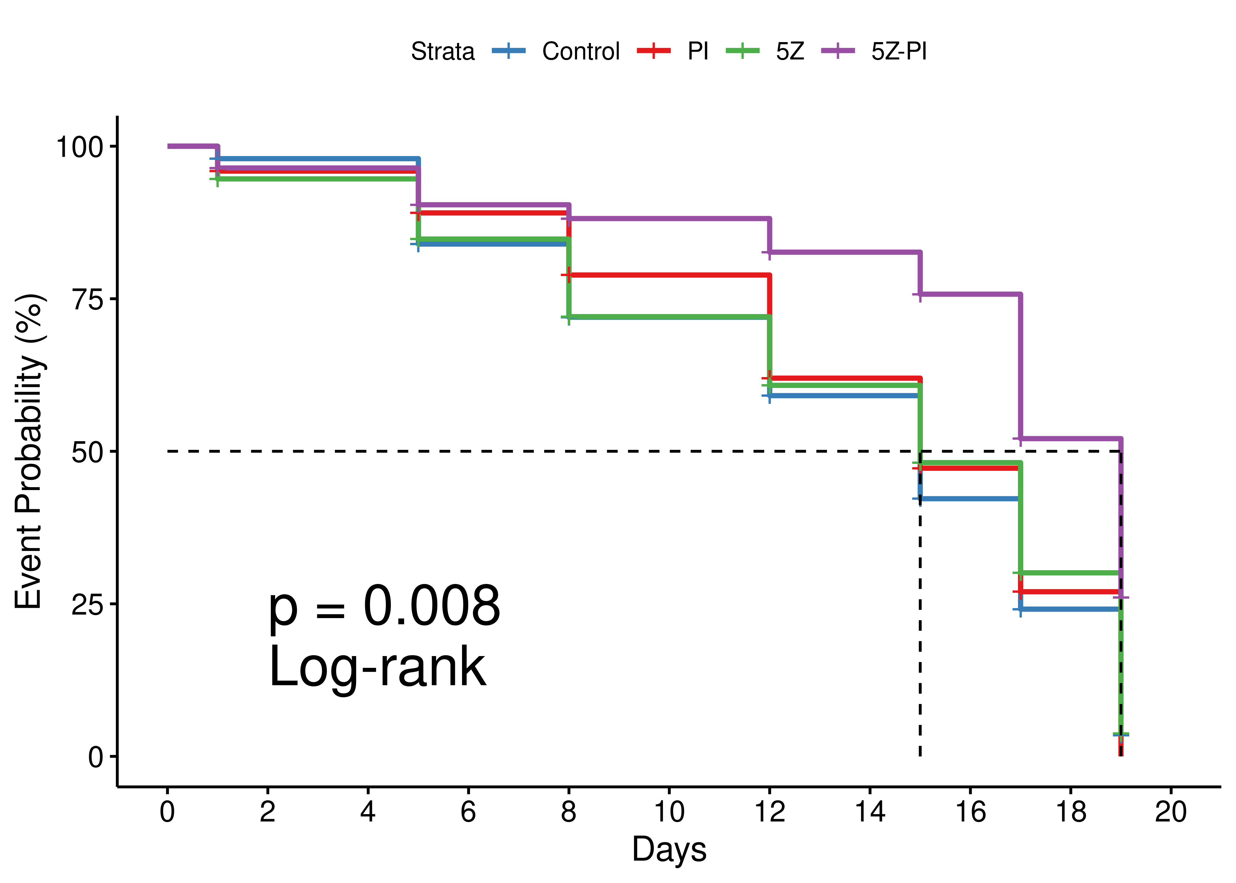
Figure 79: Mouse survival plot (Kaplan-Meier)
Mice treated with the PZ-PI drug combo have a higher survival probability compared to the individual treatment or no treatment groups.
We also compare the tumor differences between first and last day for every mouse in each respective group:
tumor_diff = tumor_data_wide %>%
  mutate(diff = `19` - `1`, rel_change = (`19`-`1`)/`1`) %>%
  mutate(drugs = factor(x = drugs, levels = c("Control", "PI", "5Z", "5Z-PI"))) %>%
  select(drugs, diff, rel_change)

# Compare single drug vs combo drug group
wilcox_res = tumor_diff %>%
  rstatix::wilcox_test(formula = diff ~ drugs,
    comparisons = list(c('5Z-PI', 'Control'), c('5Z-PI', '5Z'), c('PI','5Z-PI'))) %>%
  select(-`.y.`) %>%
  rstatix::add_xy_position()
# swap heights
y_pos = wilcox_res %>% pull(y.position)
wilcox_res$y.position = y_pos[c(3,1,2)]

set.seed(42)
tumor_diff %>%
  ggplot(aes(x = drugs, y = diff)) +
  geom_boxplot(aes(fill = drugs)) +
  geom_jitter(position = position_jitter(0.2)) +
  ggpubr::stat_pvalue_manual(wilcox_res, label = "p = {p.adj} ({p.adj.signif})") +
  scale_fill_manual(values = set1_col[c(2,1,3,4)]) +
  labs(title = 'Relative tumor size (Day 1 vs Day 19)', x = "",
    y = latex2exp::TeX('Difference in tumor volume $\\left(mm^3\\right)$')) +
  theme_classic(base_size = 14) +
    theme(plot.title = element_text(hjust = 0.5), legend.title = element_blank())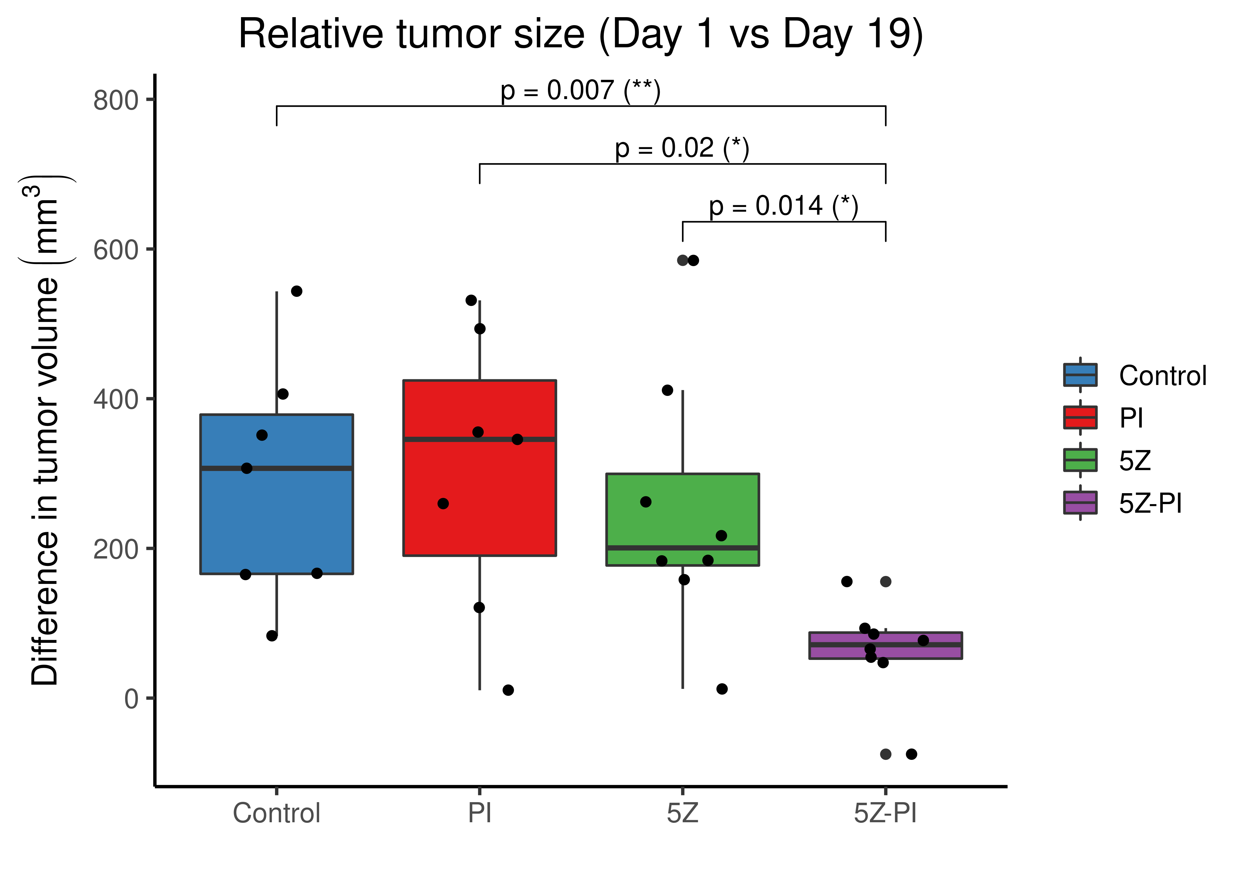
Figure 80: Comparing tumor volumes from all mice between Days 1 and 19.
We also include the table of the Wilcoxon test results between the compared groups:
DT::datatable(data = wilcox_res %>% select(1:8), options = list(searching = FALSE)) %>%
  DT::formatStyle('p.adj', backgroundColor = 'lightgreen')