Annotated Heatmaps

In this section we will use the models from the bootstrap analysis above and produce heatmaps of the models stable states and parameterization. Specifically, we will use the two CASCADE 2.0 model pools created, that have either only link-operator mutated or only topology-mutated models.

For both pools, a stable state heatmap will be produced (columns are nodes). For the first pool, the parameterization is presented with a link-operator heatmap (columns are nodes) and for the second pool as an edge heatmap (columns are edges).

Annotations

Pathways

Every node in CASCADE 2.0 belongs to a specific pathway, as can be seen in Fig. 1A of (Niederdorfer et al. 2020). The pathway categorization is a result of a computational analysis performed by the author of that paper and provided as file here.

We present the node and edge distribution across the pathways in CASCADE 2.0. For the edge pathway annotation, either both ends/nodes of an edge belong to a specific pathway and we use that label or the nodes belong to different pathways and the edge is labeled as Cross-talk:

knitr::include_graphics(path = 'img/node_path_dist.png')
knitr::include_graphics(path = 'img/edge_path_dist.png')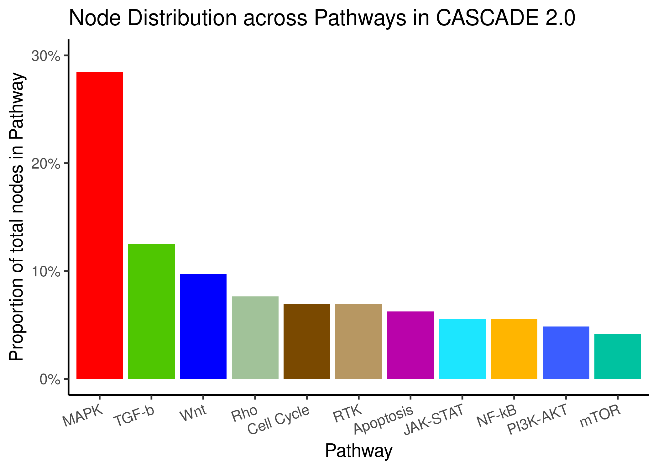

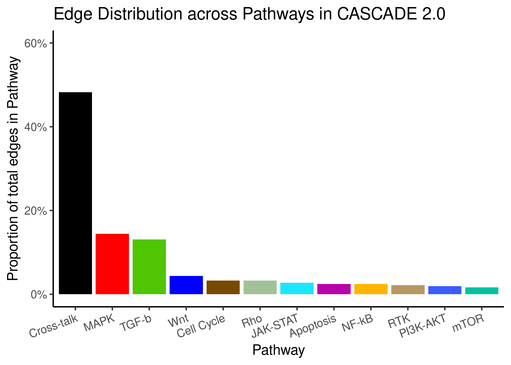
Figure 68: Node and Edge Distribution across pathways in CASCADE 2.0

\(\approx50\%\) of the edges are labeled Cross-talk
Pathways with more nodes have also more edges between these nodes

Training Data

We annotate in the stable state heatmaps the states (activation or inhibition) of the nodes as they were in the AGS training data (annotation name is Training or Calibration).

Connectivity

We annotate each node’s in-degree or out-degree connectivity for the node-oriented heatmaps, i.e. the number of its regulators (in-degree) or the number of nodes it connects to (out-degree). For the edge-oriented heatmaps, we provide either the in-degree of each edge’s target or the out-degree of each edge’s source.

Drug Target

The CASCADE 2.0 model was used to test in-silico prediction performance of the drug combination dataset in (Flobak et al. 2019). The drug panel used for the simulations involved \(18\) drugs (excluding the SF drug), each one having one to several drug targets in the CASCADE 2.0 network. We annotate this information on the combined stable states and parameterization heatmap, by specifying exactly which nodes are drug targets. For the edge-oriented heatmaps, we specify either if an edge’s target, source, both or none of them is a drug target.

COSMIC Cancer Gene Census (CGC)

We annotate some of the CASCADE 2.0 nodes either as tumor suppressors (TSG), oncogenes or both, based on the COSMIC Cancer Gene Census dataset, an expert-curated effort to describe genes driving human cancer (Sondka et al. 2018).

We used the HGNC symbols of the CASCADE 2.0 nodes and via the HGNC REST API (Braschi et al. 2019), we got the respective Ensemble IDs that helped us match the genes in the COSMIC dataset. From the COSMIC genes that we got back, we did not restrict them to a particular cancer type, we discarded the Tier 2 (lower quality) genes, as well the ones that were annotated with only the term fusion in their respective cancer role. We kept cancer genes that were annotated as both TSGs and fusion or oncogenes and fusion genes and maintained only the TSG or oncogene annotation tag (discarding only the fusion tag). Lastly note that for the CASCADE 2.0 nodes that represent families, complexes, etc. and they include a few COSMIC genes in their membership, we use a majority rule to decide which cancer role to assign to these nodes.

See the script get_cosmic_data_annot.R for more details.

A total of \(52\) CASCADE 2.0 nodes were annotated and in the following figure we can see that most of them were oncogenes, followed by TSGs and a few annotated as both categories:

knitr::include_graphics(path = 'img/cosmic_cascade2_dist.png')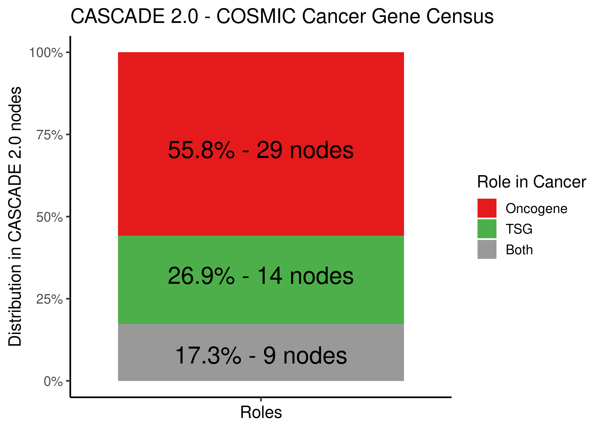

Figure 69: CASCADE 2.0 Nodes and their role in cancer as annotated by the COSMIC CGC dataset

Agreement (Parameterization vs Activity)

For the link-operator CASCADE 2.0 nodes we calculate the percent agreement between link-operator parameterization (AND-NOT => \(0\), OR-NOT => \(1\)) and stable state activity (Inhibited state => \(0\), Active state => \(1\)). The percent agreement is defined here as the number of matches (node has the link-operator AND-NOT (resp. OR-NOT) and it’s stable state activity value is \(0\) (resp. \(1\))) divided by the total amount of models (\(4500\)).

Note that the models of the link-operator Gitsbe pool from the previous bootstrap analysis that we will use for the heatmaps, had precicely \(1\) stable state each, making thus the aforementioned comparison/calculation much easier.

Link-Operator mutated models

See script lo_mutated_models_heatmaps.R for creating the heatmaps.

knitr::include_graphics(path = 'img/lo_ss_heat.png')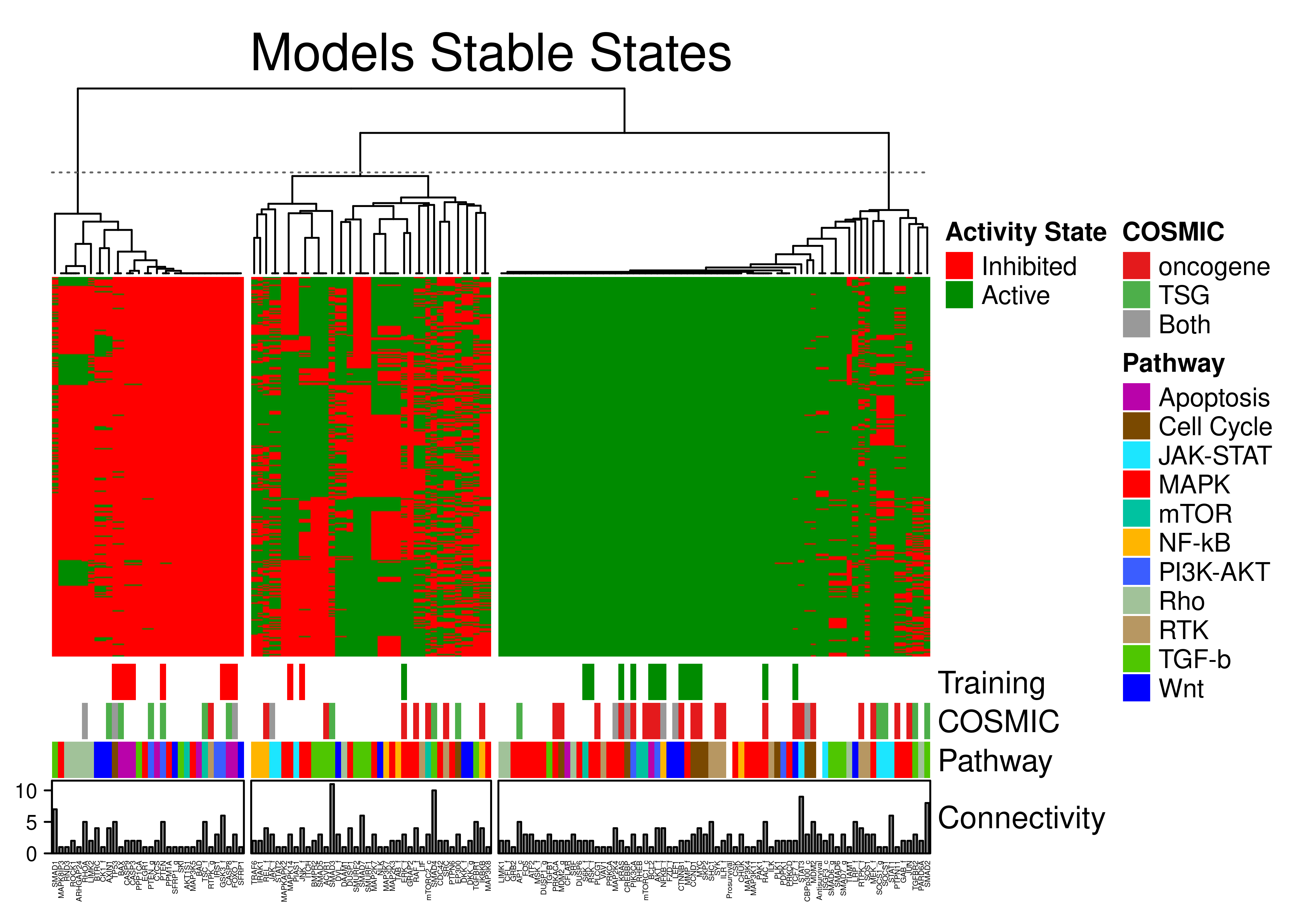

Stable state annotated heatmap for the link operator-mutated models. A total of 144 CASCADE 2.0 nodes have been grouped to 3 clusters with K-means. Training data, COSMIC, pathway and in-degree connectivity annotations are shown.

Figure 70: Stable state annotated heatmap for the link operator-mutated models. A total of 144 CASCADE 2.0 nodes have been grouped to 3 clusters with K-means. Training data, COSMIC, pathway and in-degree connectivity annotations are shown.

Calibrated models obey training data, i.e. stable states for nodes specified in training data, match the training data activity values

knitr::include_graphics(path = 'img/cosmic_state_cmp.png')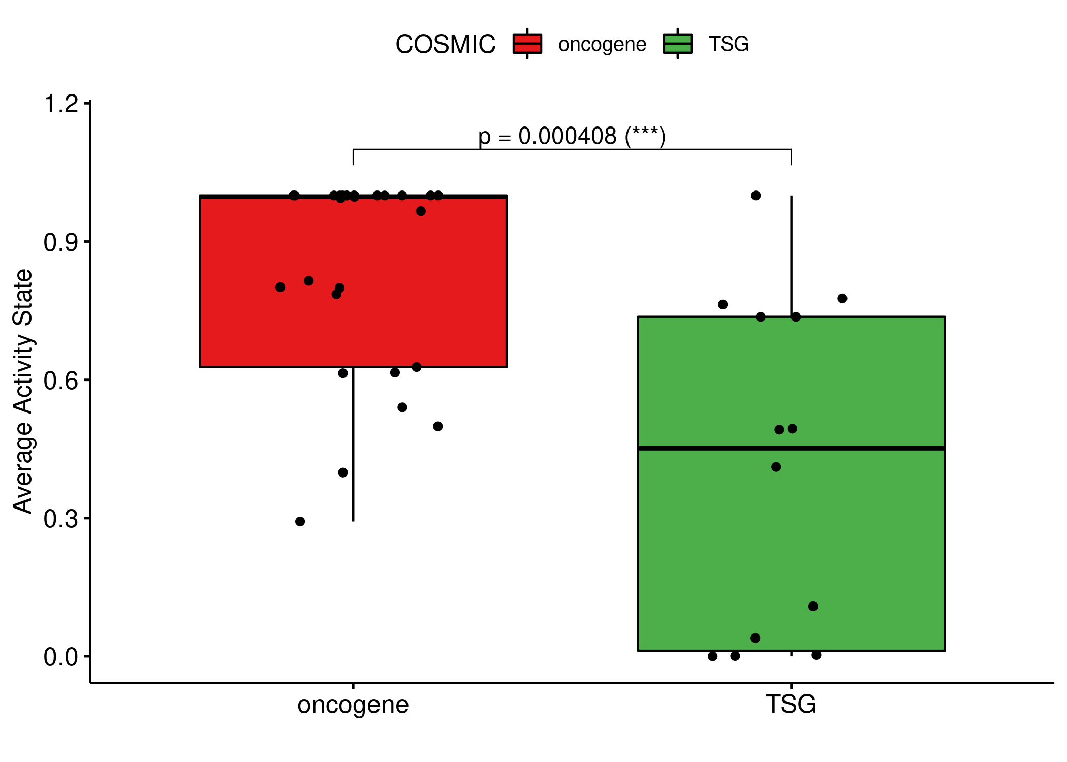

Comparing the average stable activity state between the TSG and the oncogene nodes. The Wilcoxon test is used to derive the p-value for the difference between the two groups.

Figure 71: Comparing the average stable activity state between the TSG and the oncogene nodes. The Wilcoxon test is used to derive the p-value for the difference between the two groups.

Nodes that are annotated as oncogenes have statistically higher average activity state than the ones annotated as TSGs (also evident partially from the stable states heatmap). The median values for the two groups in the boxplot are \(0.997\) (oncogene) and \(0.452\) (TSG) respectively.

The RTPK_g node is an outlier in our data: it is annotated as an oncogene and in all models it had a stable state of \(0\).

knitr::include_graphics(path = 'img/lo_heat.png')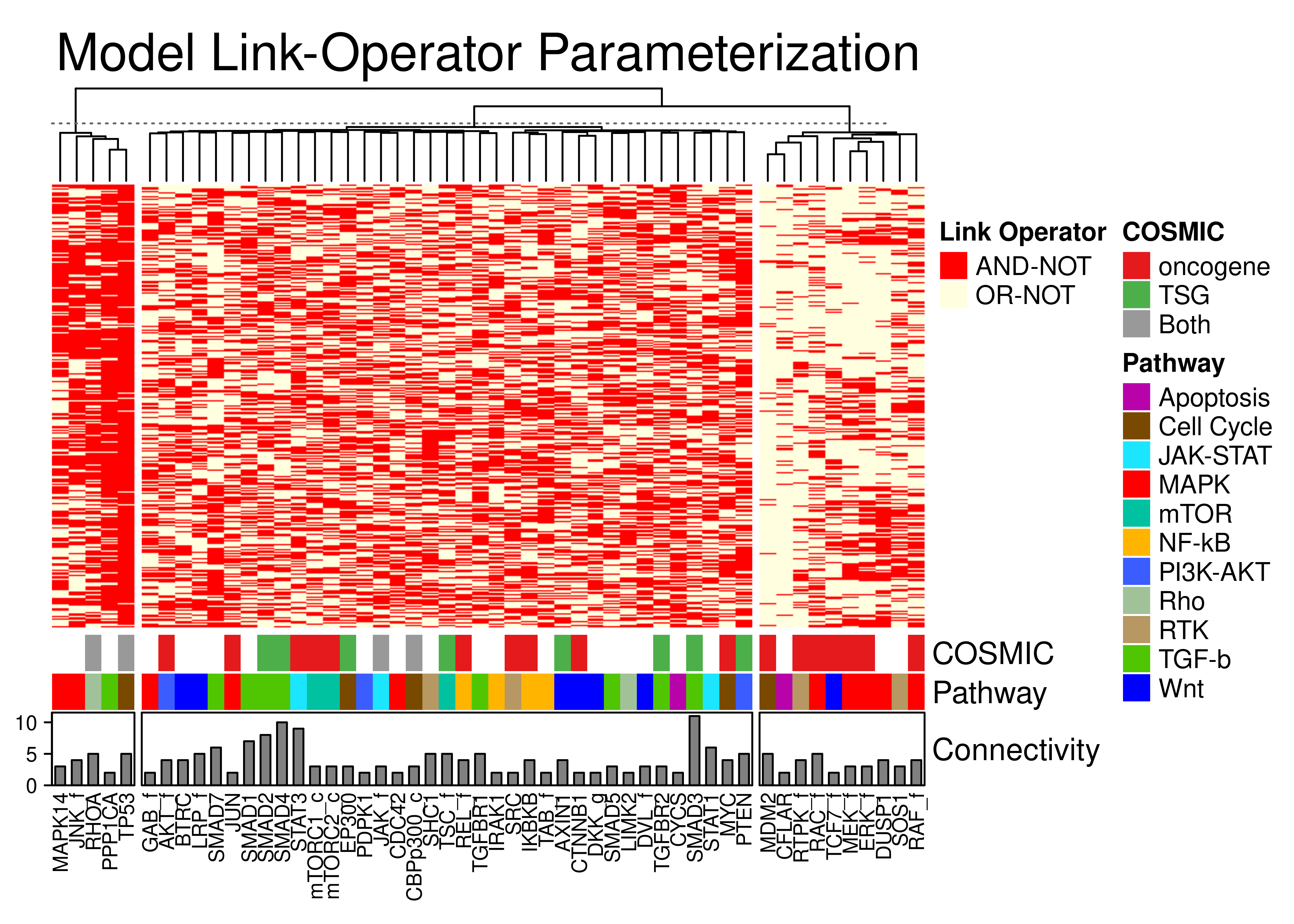

Parameterization annotated heatmap for the link operator-mutated models. Only the CASCADE 2.0 nodes that have a link-operator in their respective boolean equation are shown. The 52 link-operator nodes have been grouped to 3 clusters with K-means. COSMIC, Pathway and in-degree connectivity annotations are shown.

Figure 72: Parameterization annotated heatmap for the link operator-mutated models. Only the CASCADE 2.0 nodes that have a link-operator in their respective boolean equation are shown. The 52 link-operator nodes have been grouped to 3 clusters with K-means. COSMIC, Pathway and in-degree connectivity annotations are shown.

knitr::include_graphics(path = 'img/lo_combined_heat.png')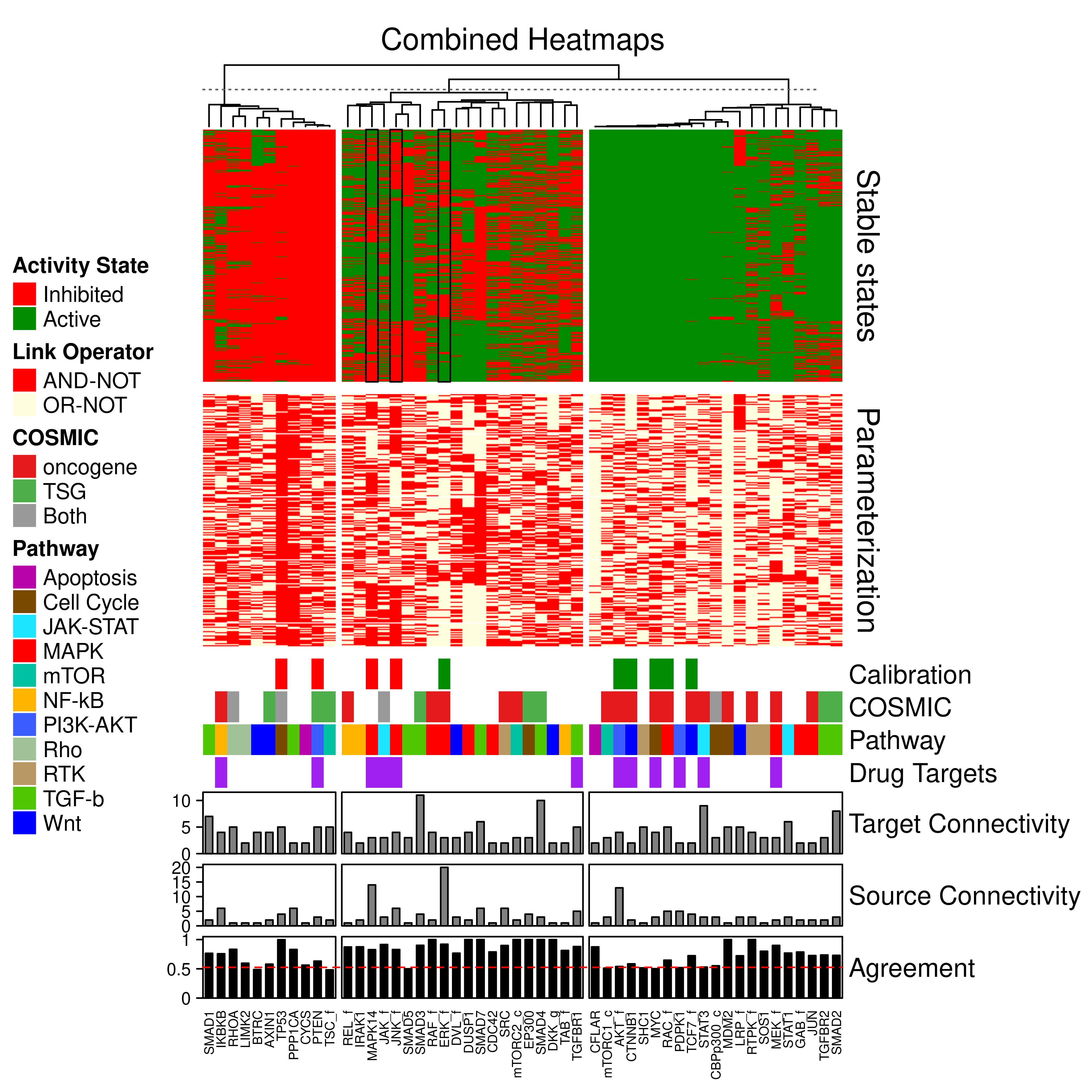

Combined stable states and parameterization heatmaps. Only the CASCADE 2.0 nodes that have a link-operator in their respective boolean equation are shown. The 52 link-operator nodes have been grouped to 3 clusters with K-means using the stable states matrix data. The link-operator data heatmap has the same row order as the stable states heatmap. Training data (Calibration), COSMIC, Pathway, Drug Target, in-degree, out-degree Connectivity and Percent Agreement annotations are shown. The stable states across the models for the JNK_f, ERK_f and MAPK14 nodes have been marked with rectangular black boxes.

Figure 73: Combined stable states and parameterization heatmaps. Only the CASCADE 2.0 nodes that have a link-operator in their respective boolean equation are shown. The 52 link-operator nodes have been grouped to 3 clusters with K-means using the stable states matrix data. The link-operator data heatmap has the same row order as the stable states heatmap. Training data (Calibration), COSMIC, Pathway, Drug Target, in-degree, out-degree Connectivity and Percent Agreement annotations are shown. The stable states across the models for the JNK_f, ERK_f and MAPK14 nodes have been marked with rectangular black boxes.

High degree of agreement between link-operator parameterization and stable state activity.

Nodes of the second cluster (the most heterogeneous one) where the parameterization and stable state activity seem to be assigned randomly (i.e. in \(\approx50\%\) of the total models a node is in an inhibited vs an active state, or has the AND-NOT vs the OR-NOT link-operator) we observe the high percent agreement scores.

In the third cluster, where the models nodes are mostly in an active state (obeying the training data), we observe that the parameterization does not affect the stable state activity and that these nodes have mostly low connectivity (\(<5\) regulators).

Topology-mutated models

See script topo_mutated_models_heatmaps.R for creating the heatmaps.

knitr::include_graphics(path = 'img/topo_ss_heat.png')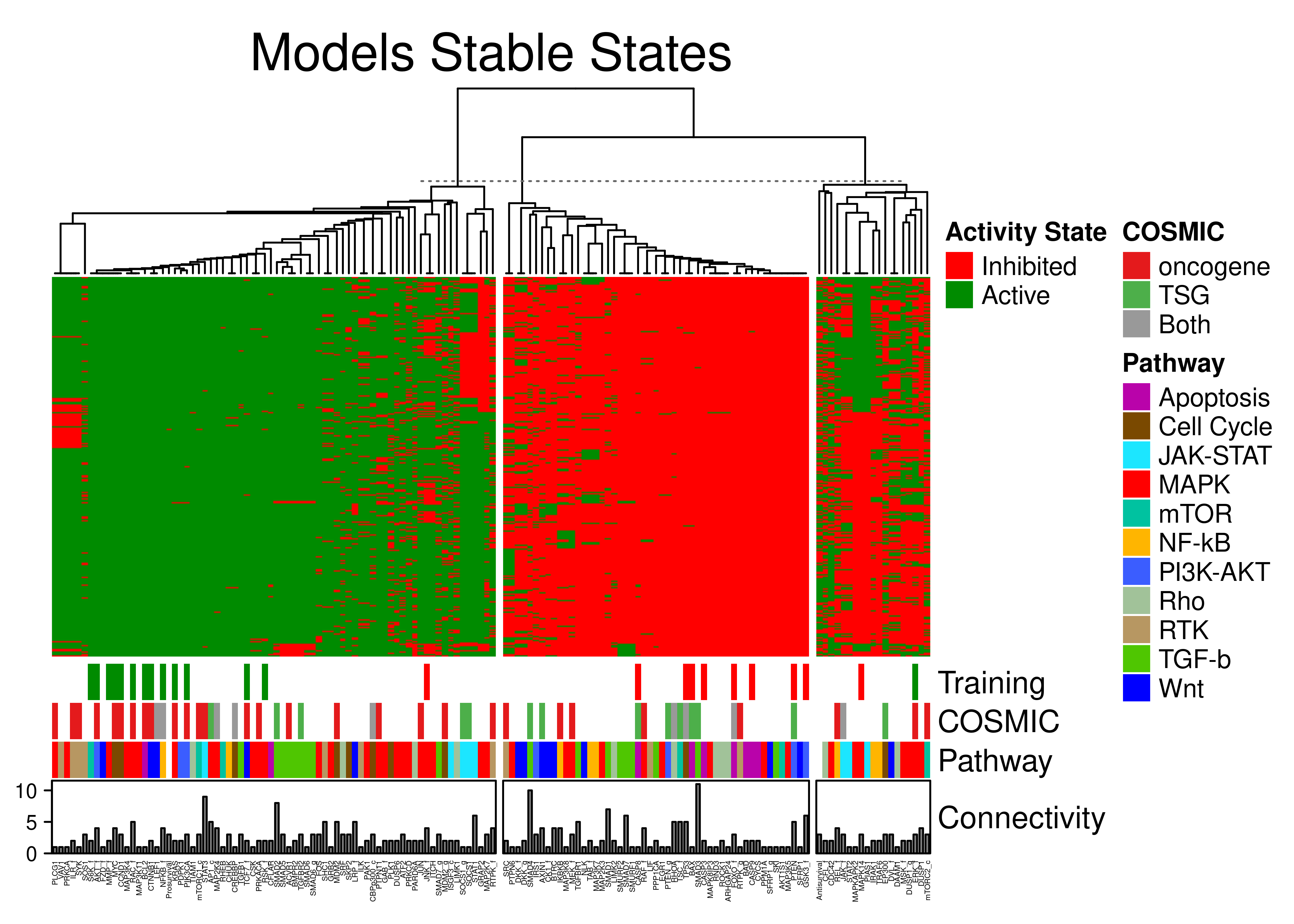

Stable state annotated heatmap for the topology-mutated models. A total of 144 CASCADE 2.0 nodes have been grouped to 3 clusters with K-means. Training data, pathway and edge target in-degree connectivity annotations are shown.

Figure 74: Stable state annotated heatmap for the topology-mutated models. A total of 144 CASCADE 2.0 nodes have been grouped to 3 clusters with K-means. Training data, pathway and edge target in-degree connectivity annotations are shown.

Calibrated models obey training data, i.e. stable states for nodes specified in training data, match the training data activity values.

knitr::include_graphics(path = 'img/edge_heat.png')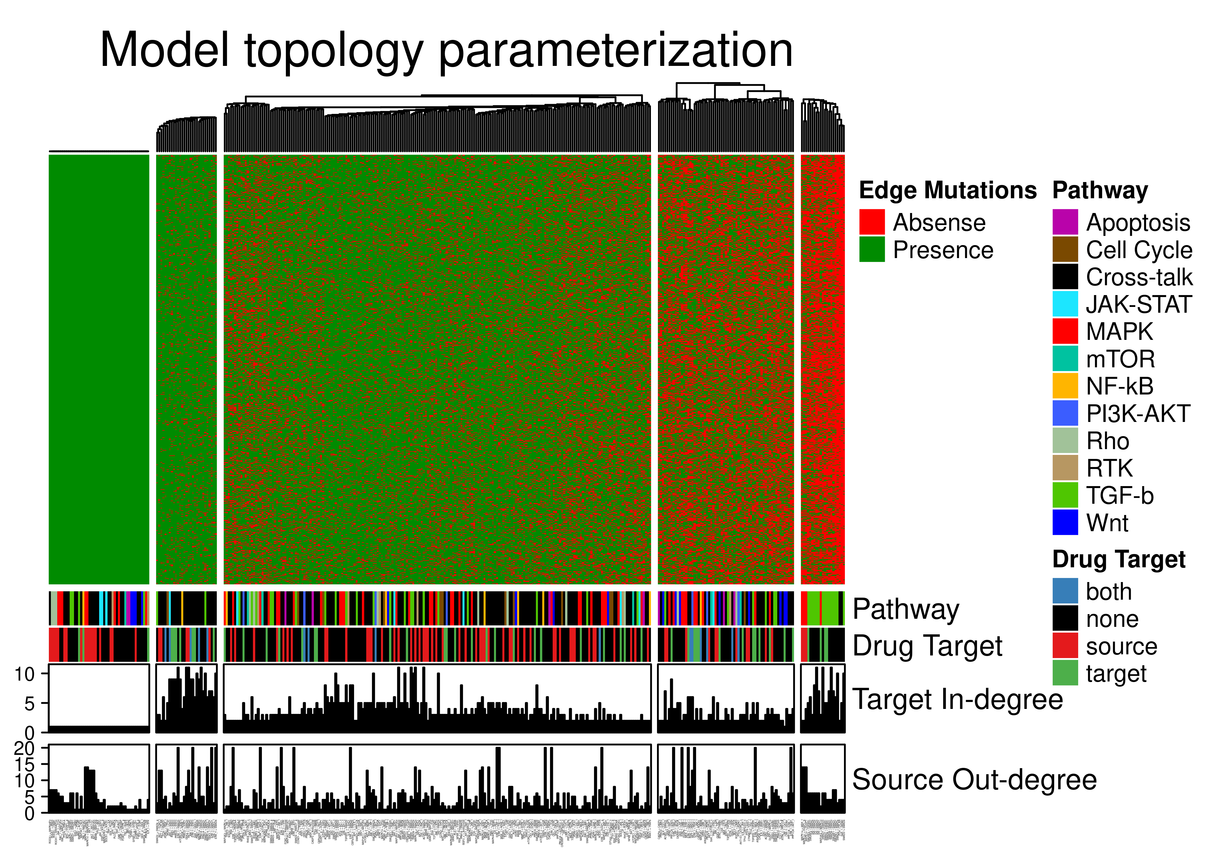

Edge annotated heatmap. All edges from the CASCADE 2.0 topology are included. A total of 367 edges have been grouped to 5 clusters with K-means. Pathway, Drug Target, edge target in-degree and edge source out-degree Connectivity annotations are shown.

Figure 75: Edge annotated heatmap. All edges from the CASCADE 2.0 topology are included. A total of 367 edges have been grouped to 5 clusters with K-means. Pathway, Drug Target, edge target in-degree and edge source out-degree Connectivity annotations are shown.

Looking at the above figure from left to right we have \(5\) clusters:

First cluster has all the edges whose target has a single regulator and these are not removed by the topology mutations in Gitsbe, to preserve the network connectivity.
Second cluster with edges that are mostly present in the topology-mutated models. These edges have two distinguished characteristics: they show high target connectivity (\(\ge 5\) regulators) - meaning that they target mostly hub-nodes - and their source and target nodes belong mostly to different pathways (i.e. they are Cross-talk edges).
Third cluster with edges that have a ~50% percent chance to stay in the topology-mutated models. These edges belong to a variety of pathways and can have both low and high target in-degree connectivity.
Fourth cluster with edges that will most likely be removed in the topology-mutated models. These edges belong to a variety of pathways and mostly have low target in-degree connectivity.
Fifth cluster with edges that are mostly absent in the topology-mutated models. Some of them are high target-connectivity nodes and most of them belong to the TGF-b pathway.

Now, we present a subset of columns (edges) of the above heatmap, chosen based on some user-defined thresholds to include only the edges that are either mostly absent or present in the models (so the second and last cluster). We do not include the edges that are present in all models (cluster 1) since there were the ones whose target had only \(1\) regulator and as such they couldn’t be removed by the Gitsbe algorithm (we don’t lose connectivity when using topology mutations).

knitr::include_graphics(path = 'img/edge_heat_stable.png')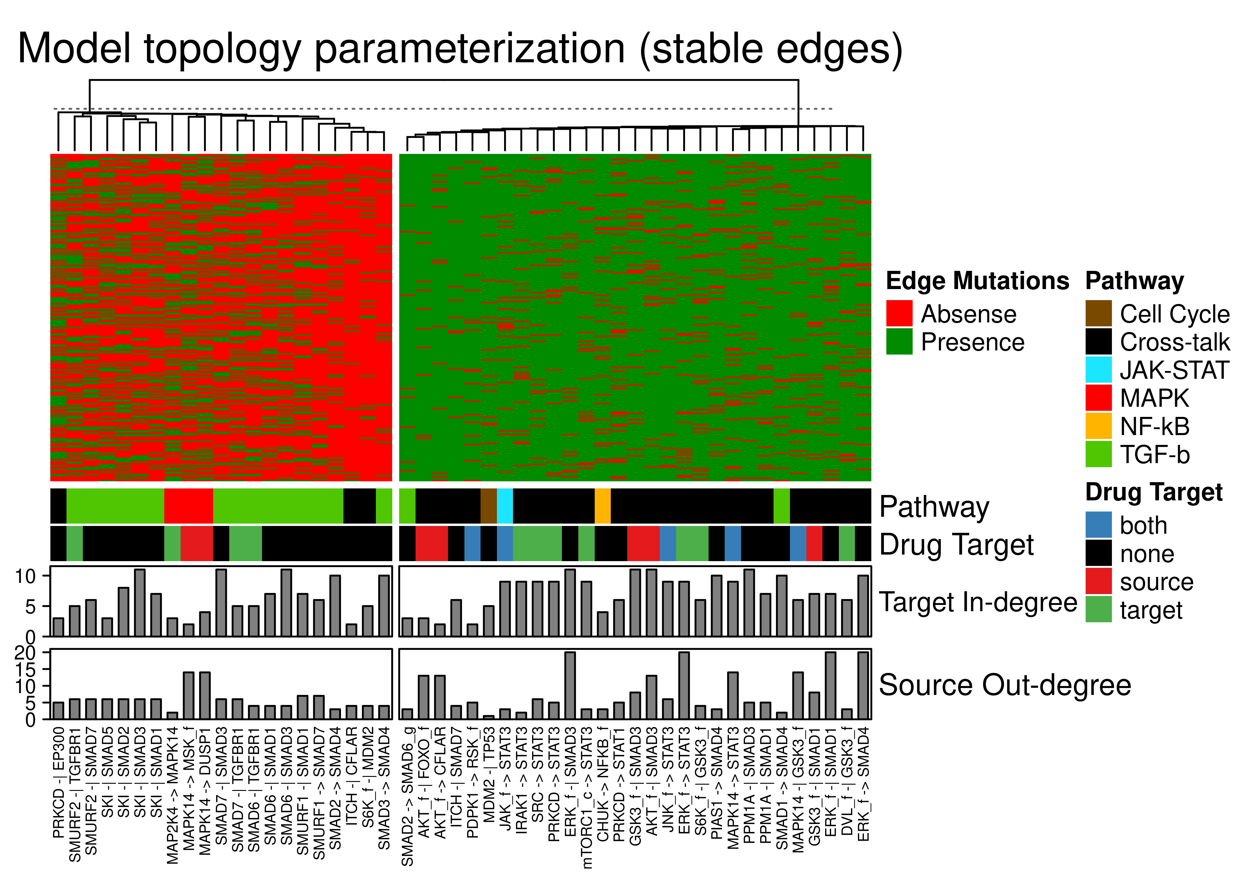

Edge annotated heatmap. A subset of the total edges is included, the least heterogeneous across all the models (rows) based on some user-defined thresholds. Edges that were always present are removed (connectivity = 1). Edges have been grouped to 2 clusters with K-means. Pathway, Drug Target, edge target in-degree and edge source out-degree Connectivity annotations are shown.

Figure 76: Edge annotated heatmap. A subset of the total edges is included, the least heterogeneous across all the models (rows) based on some user-defined thresholds. Edges that were always present are removed (connectivity = 1). Edges have been grouped to 2 clusters with K-means. Pathway, Drug Target, edge target in-degree and edge source out-degree Connectivity annotations are shown.

ERK performance investigation

We investigate the role of the activity of the ERK_f node in the performance of boolean models with link operator mutations.

In the middle cluster of the stable states heatmap (see Figure 70) there were lot of nodes whose stable state activity was different for about half of the models. For example, although ERK_f is defined in an active state in the training data, we also get models after training that have it inhibited in their corresponding stable state. Since these boolean models essentially represent AGS proliferating cancer cells, it’s remarkable that the literature curation results are also divided, i.e. around half of the publications support that activation of ERK_f and the other its inhibition (see Table S2 from (Flobak et al. 2015)). So, do we have a way to distinguish which of the two scenarios (ERK active vs inhibited) better matches the observed biological reality?

Model-wise analyses provide evidence which suggests that the overexpression of ERK_f is a characteristic biomarker of the higher performance AGS models in terms of synergy prediction, i.e. models that have ERK_f active in their stable state can predict synergies that have been observed experimentally in the AGS cancer cells.

See methodology and how to reproduce the results here.

res = readRDS(file = "data/res_erk.rds")

set1_col = RColorBrewer::brewer.pal(9, 'Set1')

stat_test_roc = res %>% 
  rstatix::wilcox_test(formula = roc_auc ~ erk_state) %>%
  rstatix::add_significance("p")

# ROC AUCs
ggboxplot(res, x = "erk_state", y = "roc_auc", fill = "erk_state", 
  palette = c(set1_col[3], set1_col[1]),
  add = "jitter", xlab = "", ylab = "ROC AUC",
  title = "ERK_f Pools Performance Comparison (ROC)") +
  scale_x_discrete(breaks = c("active","inhibited"), labels = c("Active", "Inhibited")) +
  ggpubr::stat_pvalue_manual(stat_test_roc, label = "p = {p} ({p.signif})", y.position = c(1)) +
  ylim(c(0,1)) +
  theme(plot.title = element_text(hjust = 0.5), axis.text = element_text(size = 14)) + 
  geom_hline(yintercept = 0.5, linetype = 'dashed', color = "red") +
  geom_text(aes(x = 2.1, y = 0.55, label = "Random Predictions (AUC = 0.5)")) + 
  theme(legend.position = "none")

stat_test_pr = res %>% 
  rstatix::wilcox_test(formula = pr_auc ~ erk_state) %>%
  rstatix::add_significance("p") %>%
  rstatix::add_y_position()

# PR AUCs
ggboxplot(res, x = "erk_state", y = "pr_auc", fill = "erk_state", 
  palette = c(set1_col[3], set1_col[1]),
  add = "jitter", xlab = "", ylab = "PR AUC",
  title = "ERK_f Pools Performance Comparison (Precision-Recall)") +
  scale_x_discrete(breaks = c("active","inhibited"), labels = c("Active", "Inhibited")) +
  ggpubr::stat_pvalue_manual(stat_test_pr, label = "p = {p} ({p.signif})") +
  theme(plot.title = element_text(hjust = 0.5), axis.text = element_text(size = 14)) + 
  # 6 out 153 drug combos were synergistic
  geom_hline(yintercept = 6/153, linetype = 'dashed', color = "red") +
  geom_text(aes(x = 1.05, y = 0.06, label = "Random Predictions (AUC = 0.04)")) + 
  theme(legend.position = "none")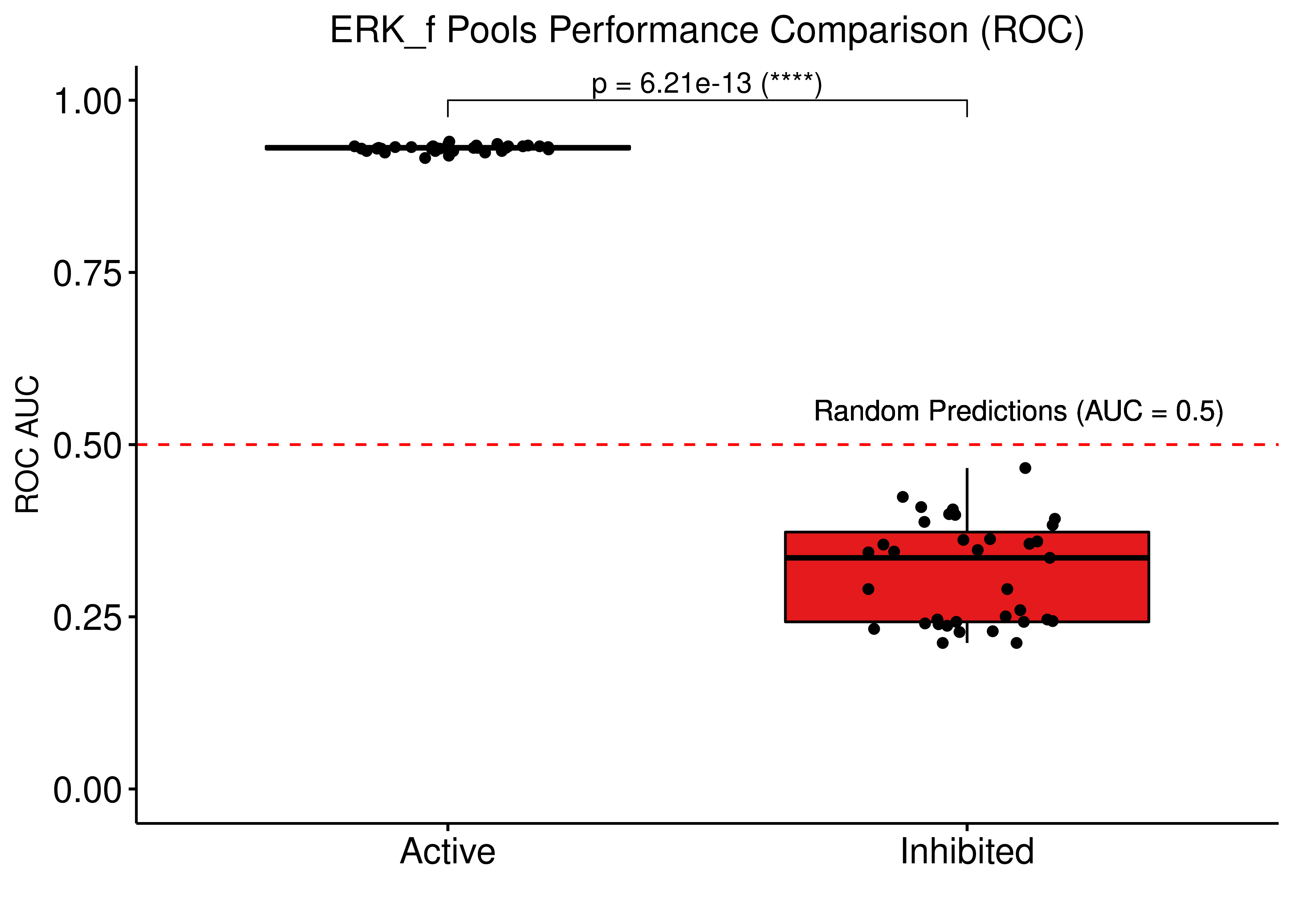

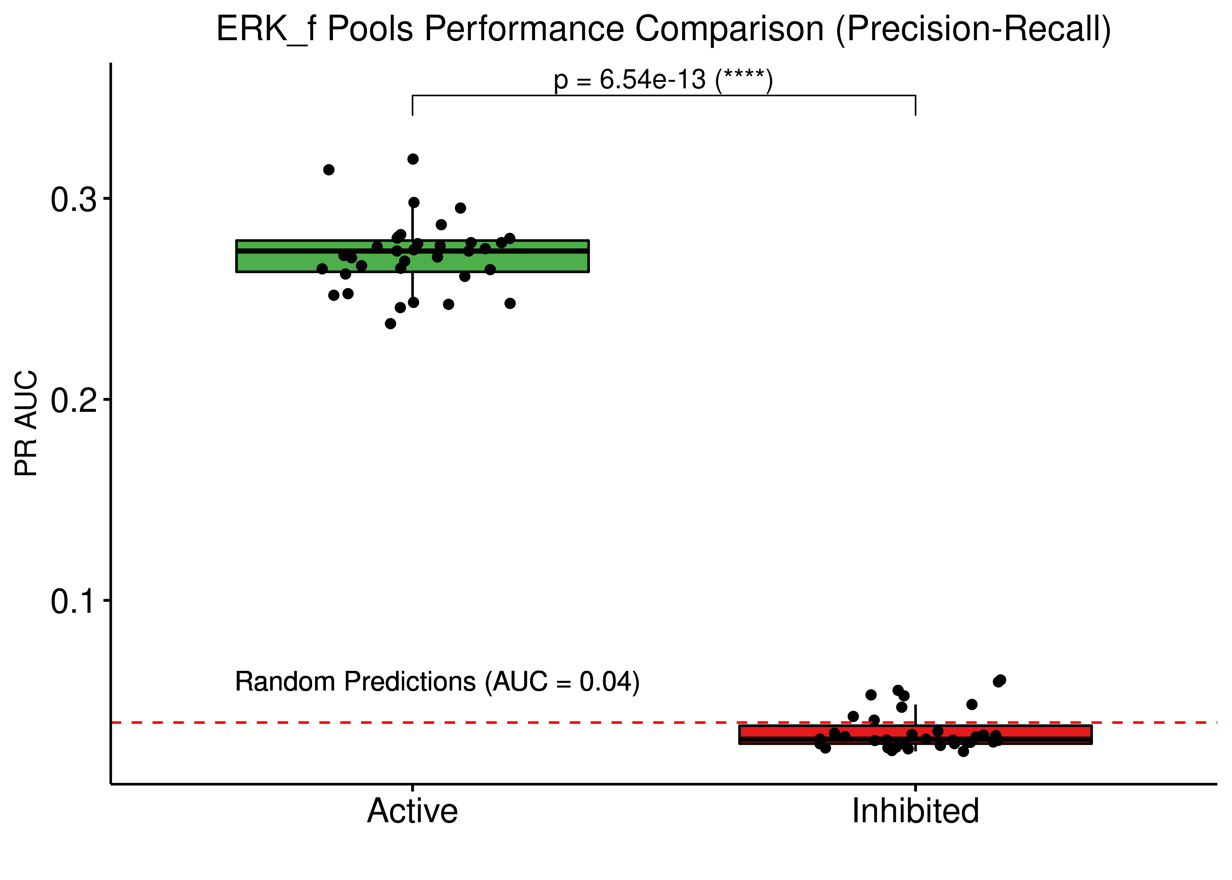
Comparing drug prediction performance (ROC and PR AUCs) between bootstrapped calibrated model ensembles from two model pools. Results were normalized to random model predictions. The models had link operator mutations only. In one pool, each model had a single stable state with ERK_f active and on the other pool ERK_f was inhibited at the stable state (CASCADE 2.0, Bliss synergy method, Ensemble-wise results)

Figure 77: Comparing drug prediction performance (ROC and PR AUCs) between bootstrapped calibrated model ensembles from two model pools. Results were normalized to random model predictions. The models had link operator mutations only. In one pool, each model had a single stable state with ERK_f active and on the other pool ERK_f was inhibited at the stable state (CASCADE 2.0, Bliss synergy method, Ensemble-wise results)

Significantly better performance of the bootstrapped ensembles with ERK_f active, suggesting that ERK should be considered active in AGS cells from a functional point of view.