CASCADE 2.0 Analysis (Topology Mutations)
Load the results:
# 'ss' => calibrated models, 'rand' => proliferative models (so not random but kind of!)
# 'ew' => ensemble-wise, 'mw' => modelwise

## HSA results ss
topo_ss_hsa_ew_50sim_file = paste0("results/topology-only/cascade_2.0_ss_50sim_fixpoints_hsa_ensemblewise_synergies.tab")
topo_ss_hsa_mw_50sim_file = paste0("results/topology-only/cascade_2.0_ss_50sim_fixpoints_hsa_modelwise_synergies.tab")
topo_ss_hsa_ew_150sim_file = paste0("results/topology-only/cascade_2.0_ss_150sim_fixpoints_hsa_ensemblewise_synergies.tab")
topo_ss_hsa_mw_150sim_file = paste0("results/topology-only/cascade_2.0_ss_150sim_fixpoints_hsa_modelwise_synergies.tab")

topo_ss_hsa_ew_synergies_50sim = emba::get_synergy_scores(topo_ss_hsa_ew_50sim_file)
topo_ss_hsa_mw_synergies_50sim = emba::get_synergy_scores(topo_ss_hsa_mw_50sim_file, file_type = "modelwise")
topo_ss_hsa_ew_synergies_150sim = emba::get_synergy_scores(topo_ss_hsa_ew_150sim_file)
topo_ss_hsa_mw_synergies_150sim = emba::get_synergy_scores(topo_ss_hsa_mw_150sim_file, file_type = "modelwise")

## HSA results rand
topo_prolif_hsa_ew_50sim_file = paste0("results/topology-only/cascade_2.0_rand_50sim_fixpoints_hsa_ensemblewise_synergies.tab")
topo_prolif_hsa_mw_50sim_file = paste0("results/topology-only/cascade_2.0_rand_50sim_fixpoints_hsa_modelwise_synergies.tab")
topo_prolif_hsa_ew_150sim_file = paste0("results/topology-only/cascade_2.0_rand_150sim_fixpoints_hsa_ensemblewise_synergies.tab")
topo_prolif_hsa_mw_150sim_file = paste0("results/topology-only/cascade_2.0_rand_150sim_fixpoints_hsa_modelwise_synergies.tab")

topo_prolif_hsa_ew_synergies_50sim = emba::get_synergy_scores(topo_prolif_hsa_ew_50sim_file)
topo_prolif_hsa_mw_synergies_50sim = emba::get_synergy_scores(topo_prolif_hsa_mw_50sim_file, file_type = "modelwise")
topo_prolif_hsa_ew_synergies_150sim = emba::get_synergy_scores(topo_prolif_hsa_ew_150sim_file)
topo_prolif_hsa_mw_synergies_150sim = emba::get_synergy_scores(topo_prolif_hsa_mw_150sim_file, file_type = "modelwise")

## Bliss results ss
topo_ss_bliss_ew_50sim_file = paste0("results/topology-only/cascade_2.0_ss_50sim_fixpoints_bliss_ensemblewise_synergies.tab")
topo_ss_bliss_mw_50sim_file = paste0("results/topology-only/cascade_2.0_ss_50sim_fixpoints_bliss_modelwise_synergies.tab")
topo_ss_bliss_ew_150sim_file = paste0("results/topology-only/cascade_2.0_ss_150sim_fixpoints_bliss_ensemblewise_synergies.tab")
topo_ss_bliss_mw_150sim_file = paste0("results/topology-only/cascade_2.0_ss_150sim_fixpoints_bliss_modelwise_synergies.tab")

topo_ss_bliss_ew_synergies_50sim = emba::get_synergy_scores(topo_ss_bliss_ew_50sim_file)
topo_ss_bliss_mw_synergies_50sim = emba::get_synergy_scores(topo_ss_bliss_mw_50sim_file, file_type = "modelwise")
topo_ss_bliss_ew_synergies_150sim = emba::get_synergy_scores(topo_ss_bliss_ew_150sim_file)
topo_ss_bliss_mw_synergies_150sim = emba::get_synergy_scores(topo_ss_bliss_mw_150sim_file, file_type = "modelwise")

## Bliss results rand
topo_prolif_bliss_ew_50sim_file = paste0("results/topology-only/cascade_2.0_rand_50sim_fixpoints_bliss_ensemblewise_synergies.tab")
topo_prolif_bliss_mw_50sim_file = paste0("results/topology-only/cascade_2.0_rand_50sim_fixpoints_bliss_modelwise_synergies.tab")
topo_prolif_bliss_ew_150sim_file = paste0("results/topology-only/cascade_2.0_rand_150sim_fixpoints_bliss_ensemblewise_synergies.tab")
topo_prolif_bliss_mw_150sim_file = paste0("results/topology-only/cascade_2.0_rand_150sim_fixpoints_bliss_modelwise_synergies.tab")

topo_prolif_bliss_ew_synergies_50sim = emba::get_synergy_scores(topo_prolif_bliss_ew_50sim_file)
topo_prolif_bliss_mw_synergies_50sim = emba::get_synergy_scores(topo_prolif_bliss_mw_50sim_file, file_type = "modelwise")
topo_prolif_bliss_ew_synergies_150sim = emba::get_synergy_scores(topo_prolif_bliss_ew_150sim_file)
topo_prolif_bliss_mw_synergies_150sim = emba::get_synergy_scores(topo_prolif_bliss_mw_150sim_file, file_type = "modelwise")

# calculate probability of synergy in the modelwise results
topo_ss_hsa_mw_synergies_50sim = topo_ss_hsa_mw_synergies_50sim %>%
  mutate(synergy_prob_ss = synergies/(synergies + `non-synergies`))
topo_ss_hsa_mw_synergies_150sim = topo_ss_hsa_mw_synergies_150sim %>%
  mutate(synergy_prob_ss = synergies/(synergies + `non-synergies`))
topo_prolif_hsa_mw_synergies_50sim = topo_prolif_hsa_mw_synergies_50sim %>%
  mutate(synergy_prob_ss = synergies/(synergies + `non-synergies`))
topo_prolif_hsa_mw_synergies_150sim = topo_prolif_hsa_mw_synergies_150sim %>%
  mutate(synergy_prob_ss = synergies/(synergies + `non-synergies`))
topo_ss_bliss_mw_synergies_50sim = topo_ss_bliss_mw_synergies_50sim %>%
  mutate(synergy_prob_ss = synergies/(synergies + `non-synergies`))
topo_ss_bliss_mw_synergies_150sim = topo_ss_bliss_mw_synergies_150sim %>%
  mutate(synergy_prob_ss = synergies/(synergies + `non-synergies`))
topo_prolif_bliss_mw_synergies_50sim = topo_prolif_bliss_mw_synergies_50sim %>%
  mutate(synergy_prob_ss = synergies/(synergies + `non-synergies`))
topo_prolif_bliss_mw_synergies_150sim = topo_prolif_bliss_mw_synergies_150sim %>%
  mutate(synergy_prob_ss = synergies/(synergies + `non-synergies`))

# Tidy the data
pred_topo_ew_hsa = bind_cols(
  topo_ss_hsa_ew_synergies_50sim %>% rename(ss_score_50sim = score),
  topo_ss_hsa_ew_synergies_150sim %>% select(score) %>% rename(ss_score_150sim = score),
  topo_prolif_hsa_ew_synergies_50sim %>% select(score) %>% rename(prolif_score_50sim = score),
  topo_prolif_hsa_ew_synergies_150sim %>% select(score) %>% rename(prolif_score_150sim = score),
  as_tibble_col(observed, column_name = "observed"))

pred_topo_mw_hsa = bind_cols(
  topo_ss_hsa_mw_synergies_50sim %>% select(perturbation, synergy_prob_ss) %>% rename(synergy_prob_ss_50sim = synergy_prob_ss),
  topo_ss_hsa_mw_synergies_150sim %>% select(synergy_prob_ss) %>% rename(synergy_prob_ss_150sim = synergy_prob_ss),
  topo_prolif_hsa_mw_synergies_50sim %>% select(synergy_prob_ss) %>% rename(synergy_prob_prolif_50sim = synergy_prob_ss),
  topo_prolif_hsa_mw_synergies_150sim %>% select(synergy_prob_ss) %>% rename(synergy_prob_prolif_150sim = synergy_prob_ss),
  as_tibble_col(observed, column_name = "observed"))

pred_topo_ew_bliss = bind_cols(
  topo_ss_bliss_ew_synergies_50sim %>% rename(ss_score_50sim = score),
  topo_ss_bliss_ew_synergies_150sim %>% select(score) %>% rename(ss_score_150sim = score),
  topo_prolif_bliss_ew_synergies_50sim %>% select(score) %>% rename(prolif_score_50sim = score),
  topo_prolif_bliss_ew_synergies_150sim %>% select(score) %>% rename(prolif_score_150sim = score),
  as_tibble_col(observed, column_name = "observed"))

pred_topo_mw_bliss = bind_cols(
  topo_ss_bliss_mw_synergies_50sim %>% select(perturbation, synergy_prob_ss) %>% rename(synergy_prob_ss_50sim = synergy_prob_ss),
  topo_ss_bliss_mw_synergies_150sim %>% select(synergy_prob_ss) %>% rename(synergy_prob_ss_150sim = synergy_prob_ss),
  topo_prolif_bliss_mw_synergies_50sim %>% select(synergy_prob_ss) %>% rename(synergy_prob_prolif_50sim = synergy_prob_ss),
  topo_prolif_bliss_mw_synergies_150sim %>% select(synergy_prob_ss) %>% rename(synergy_prob_prolif_150sim = synergy_prob_ss),
  as_tibble_col(observed, column_name = "observed"))
HSA Results
- HSA refers to the synergy method used in
Drabmeto assess the synergies from thegitsbemodels - We test performance using ROC and PR AUC for both the ensemble-wise and model-wise synergies from
Drabme - Calibrated models: fitted to steady state (\(50,150\) simulations)
- Random models: fitted to proliferation profile (\(50,150\) simulations)
Gitsbemodels have only topology mutations (\(50\) mutations as a bootstrap value, \(10\) after models with stable states are found)
ROC curves
topo_res_ss_ew_50sim = get_roc_stats(df = pred_topo_ew_hsa, pred_col = "ss_score_50sim", label_col = "observed")
topo_res_ss_ew_150sim = get_roc_stats(df = pred_topo_ew_hsa, pred_col = "ss_score_150sim", label_col = "observed")
topo_res_prolif_ew_50sim = get_roc_stats(df = pred_topo_ew_hsa, pred_col = "prolif_score_50sim", label_col = "observed")
topo_res_prolif_ew_150sim = get_roc_stats(df = pred_topo_ew_hsa, pred_col = "prolif_score_150sim", label_col = "observed")

topo_res_ss_mw_50sim = get_roc_stats(df = pred_topo_mw_hsa, pred_col = "synergy_prob_ss_50sim", label_col = "observed", direction = ">")
topo_res_ss_mw_150sim = get_roc_stats(df = pred_topo_mw_hsa, pred_col = "synergy_prob_ss_150sim", label_col = "observed", direction = ">")
topo_res_prolif_mw_50sim = get_roc_stats(df = pred_topo_mw_hsa, pred_col = "synergy_prob_prolif_50sim", label_col = "observed", direction = ">")
topo_res_prolif_mw_150sim = get_roc_stats(df = pred_topo_mw_hsa, pred_col = "synergy_prob_prolif_150sim", label_col = "observed", direction = ">")

# Plot ROCs
plot(x = topo_res_ss_ew_50sim$roc_stats$FPR, y = topo_res_ss_ew_50sim$roc_stats$TPR,
  type = 'l', lwd = 3, col = my_palette[1], main = 'ROC curve, Ensemble-wise synergies (HSA)',
  xlab = 'False Positive Rate (FPR)', ylab = 'True Positive Rate (TPR)')
lines(x = topo_res_ss_ew_150sim$roc_stats$FPR, y = topo_res_ss_ew_150sim$roc_stats$TPR,
  lwd = 3, col = my_palette[2])
lines(x = topo_res_prolif_ew_50sim$roc_stats$FPR, y = topo_res_prolif_ew_50sim$roc_stats$TPR,
  lwd = 3, col = my_palette[3])
lines(x = topo_res_prolif_ew_150sim$roc_stats$FPR, y = topo_res_prolif_ew_150sim$roc_stats$TPR,
  lwd = 3, col = my_palette[4])
legend('bottomright', title = 'AUC', col = my_palette[1:4], pch = 19,
  legend = c(paste(round(topo_res_ss_ew_50sim$AUC, digits = 2), "Calibrated (50 sim)"),
    paste(round(topo_res_ss_ew_150sim$AUC, digits = 2), "Calibrated (150 sim)"),
    paste(round(topo_res_prolif_ew_50sim$AUC, digits = 2), "Random (50 sim)"),
    paste(round(topo_res_prolif_ew_150sim$AUC, digits = 2), "Random (150 sim)")))
grid(lwd = 0.5)
abline(a = 0, b = 1, col = 'lightgrey', lty = 'dotdash', lwd = 1.2)

plot(x = topo_res_ss_mw_50sim$roc_stats$FPR, y = topo_res_ss_mw_50sim$roc_stats$TPR,
  type = 'l', lwd = 3, col = my_palette[1], main = 'ROC curve, Model-wise synergies (HSA)',
  xlab = 'False Positive Rate (FPR)', ylab = 'True Positive Rate (TPR)')
lines(x = topo_res_ss_mw_150sim$roc_stats$FPR, y = topo_res_ss_mw_150sim$roc_stats$TPR,
  lwd = 3, col = my_palette[2])
lines(x = topo_res_prolif_mw_50sim$roc_stats$FPR, y = topo_res_prolif_mw_50sim$roc_stats$TPR,
  lwd = 3, col = my_palette[3])
lines(x = topo_res_prolif_mw_150sim$roc_stats$FPR, y = topo_res_prolif_mw_150sim$roc_stats$TPR,
  lwd = 3, col = my_palette[4])
legend('bottomright', title = 'AUC', col = my_palette[1:4], pch = 19,
  legend = c(paste(round(topo_res_ss_mw_50sim$AUC, digits = 2), "Calibrated (50 sim)"),
    paste(round(topo_res_ss_mw_150sim$AUC, digits = 2), "Calibrated (150 sim)"),
    paste(round(topo_res_prolif_mw_50sim$AUC, digits = 2), "Random (50 sim)"),
    paste(round(topo_res_prolif_mw_150sim$AUC, digits = 2), "Random (150 sim)")))
grid(lwd = 0.5)
abline(a = 0, b = 1, col = 'lightgrey', lty = 'dotdash', lwd = 1.2)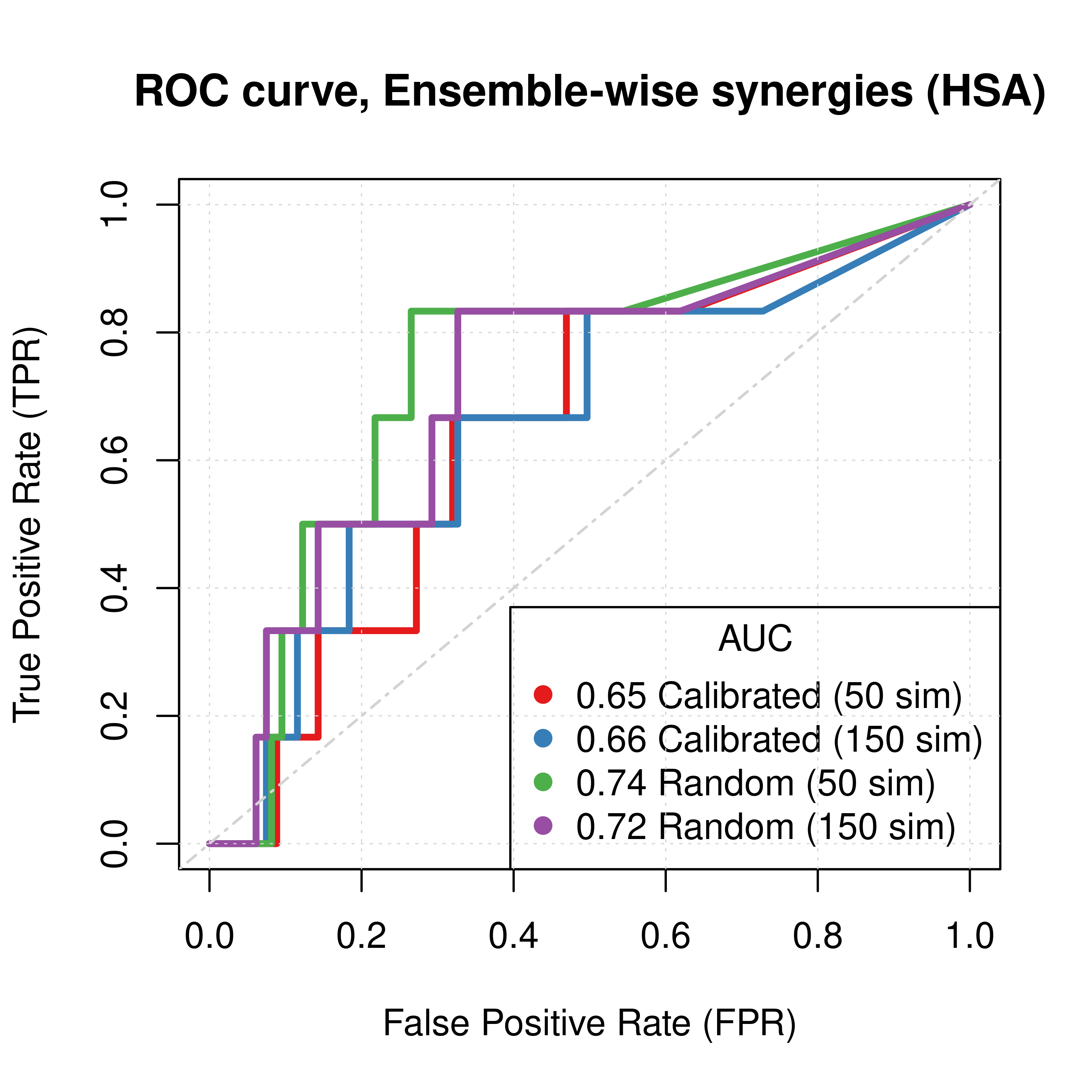
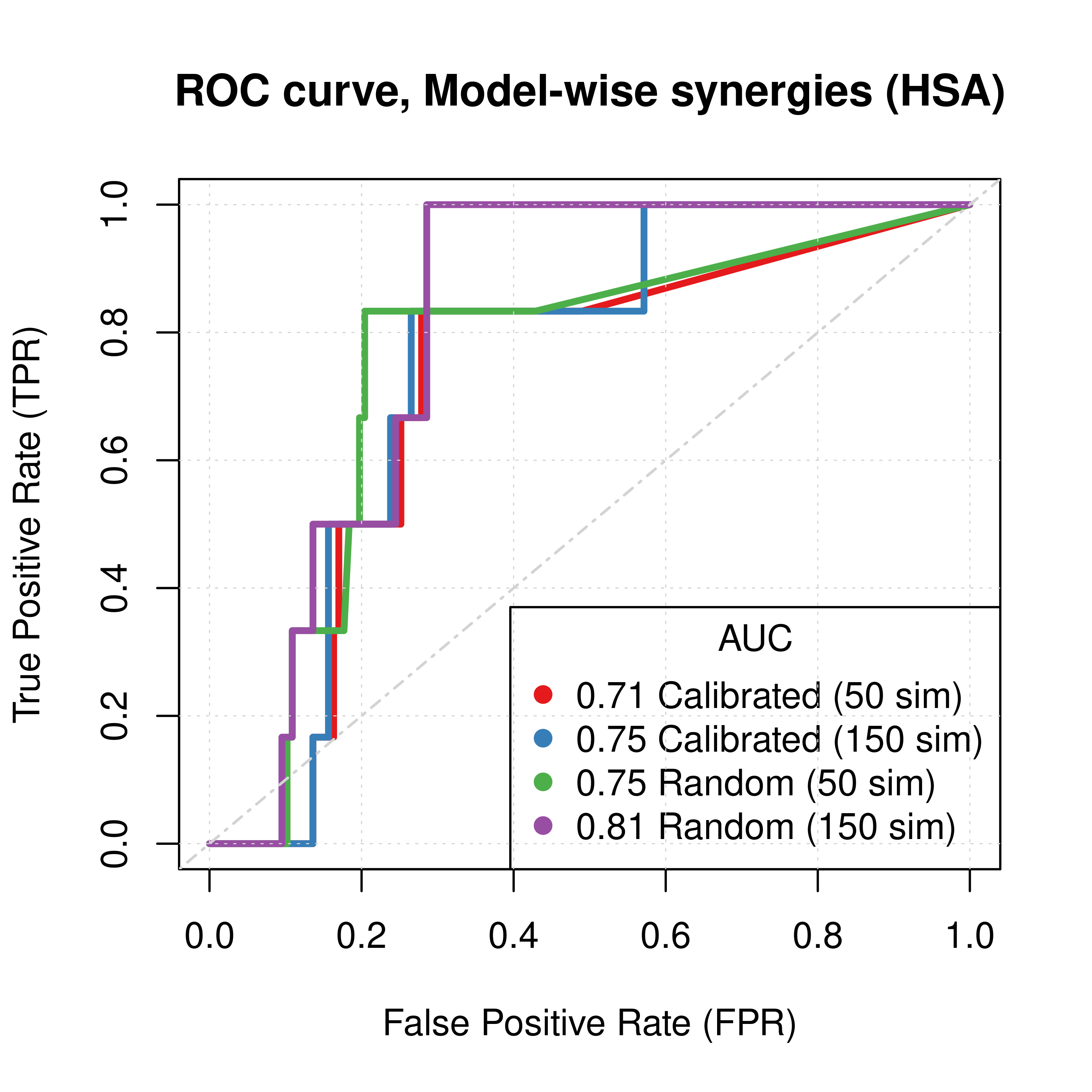
Figure 49: ROC curves (CASCADE 2.0, Topology Mutations, HSA synergy method)
PR curves
pr_topo_res_ss_ew_50sim = pr.curve(scores.class0 = pred_topo_ew_hsa %>% pull(ss_score_50sim) %>% (function(x) {-x}),
  weights.class0 = pred_topo_ew_hsa %>% pull(observed), curve = TRUE, rand.compute = TRUE)
pr_topo_res_ss_ew_150sim = pr.curve(scores.class0 = pred_topo_ew_hsa %>% pull(ss_score_150sim) %>% (function(x) {-x}),
  weights.class0 = pred_topo_ew_hsa %>% pull(observed), curve = TRUE)
pr_topo_res_prolif_ew_50sim = pr.curve(scores.class0 = pred_topo_ew_hsa %>% pull(prolif_score_50sim) %>% (function(x) {-x}),
  weights.class0 = pred_topo_ew_hsa %>% pull(observed), curve = TRUE)
pr_topo_res_prolif_ew_150sim = pr.curve(scores.class0 = pred_topo_ew_hsa %>% pull(prolif_score_150sim) %>% (function(x) {-x}),
  weights.class0 = pred_topo_ew_hsa %>% pull(observed), curve = TRUE)

pr_topo_res_ss_mw_50sim = pr.curve(scores.class0 = pred_topo_mw_hsa %>% pull(synergy_prob_ss_50sim),
  weights.class0 = pred_topo_mw_hsa %>% pull(observed), curve = TRUE, rand.compute = TRUE)
pr_topo_res_ss_mw_150sim = pr.curve(scores.class0 = pred_topo_mw_hsa %>% pull(synergy_prob_ss_150sim),
  weights.class0 = pred_topo_mw_hsa %>% pull(observed), curve = TRUE)
pr_topo_res_prolif_mw_50sim = pr.curve(scores.class0 = pred_topo_mw_hsa %>% pull(synergy_prob_prolif_50sim),
  weights.class0 = pred_topo_mw_hsa %>% pull(observed), curve = TRUE)
pr_topo_res_prolif_mw_150sim = pr.curve(scores.class0 = pred_topo_mw_hsa %>% pull(synergy_prob_prolif_150sim),
  weights.class0 = pred_topo_mw_hsa %>% pull(observed), curve = TRUE)

plot(pr_topo_res_ss_ew_50sim, main = 'PR curve, Ensemble-wise synergies (HSA)',
  auc.main = FALSE, color = my_palette[1], rand.plot = TRUE)
plot(pr_topo_res_ss_ew_150sim, add = TRUE, color = my_palette[2])
plot(pr_topo_res_prolif_ew_50sim, add = TRUE, color = my_palette[3])
plot(pr_topo_res_prolif_ew_150sim, add = TRUE, color = my_palette[4])
legend('topright', title = 'AUC', col = my_palette[1:4], pch = 19,
  legend = c(paste(round(pr_topo_res_ss_ew_50sim$auc.davis.goadrich, digits = 3), "Calibrated (50 sim)"),
    paste(round(pr_topo_res_ss_ew_150sim$auc.davis.goadrich, digits = 3), "Calibrated (150 sim)"),
    paste(round(pr_topo_res_prolif_ew_50sim$auc.davis.goadrich, digits = 3), "Random (50 sim)"),
    paste(round(pr_topo_res_prolif_ew_150sim$auc.davis.goadrich, digits = 3), "Random (150 sim)")))
grid(lwd = 0.5)

plot(pr_topo_res_ss_mw_50sim, main = 'PR curve, Model-wise synergies (HSA)',
  auc.main = FALSE, color = my_palette[1], rand.plot = TRUE)
plot(pr_topo_res_ss_mw_150sim, add = TRUE, color = my_palette[2])
plot(pr_topo_res_prolif_mw_50sim, add = TRUE, color = my_palette[3])
plot(pr_topo_res_prolif_mw_150sim, add = TRUE, color = my_palette[4])
legend('topright', title = 'AUC', col = my_palette[1:4], pch = 19,
  legend = c(paste(round(pr_topo_res_ss_mw_50sim$auc.davis.goadrich, digits = 3), "Calibrated (50 sim)"),
    paste(round(pr_topo_res_ss_mw_150sim$auc.davis.goadrich, digits = 3), "Calibrated (150 sim)"),
    paste(round(pr_topo_res_prolif_mw_50sim$auc.davis.goadrich, digits = 3), "Random (50 sim)"),
    paste(round(pr_topo_res_prolif_mw_150sim$auc.davis.goadrich, digits = 3), "Random (150 sim)")))
grid(lwd = 0.5)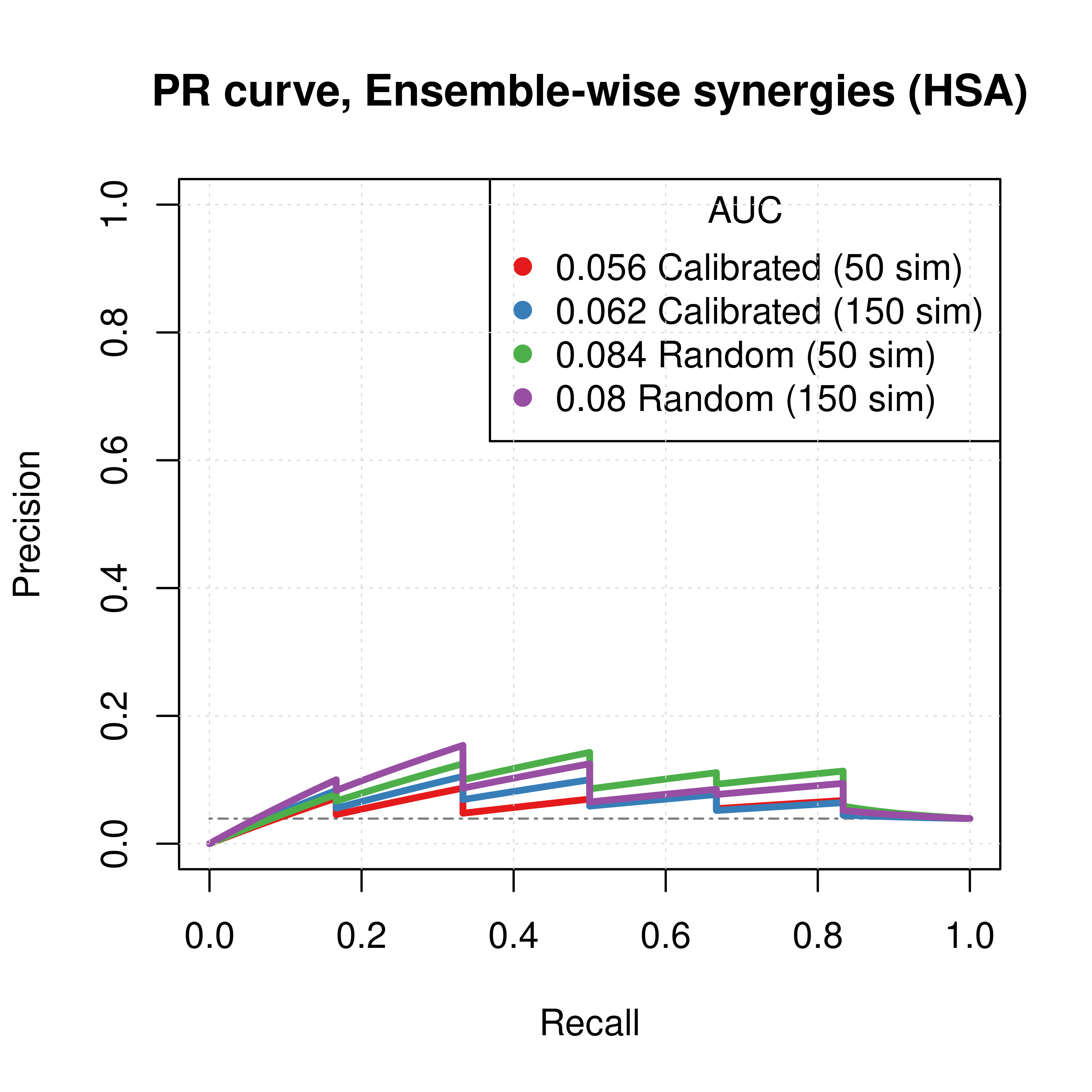
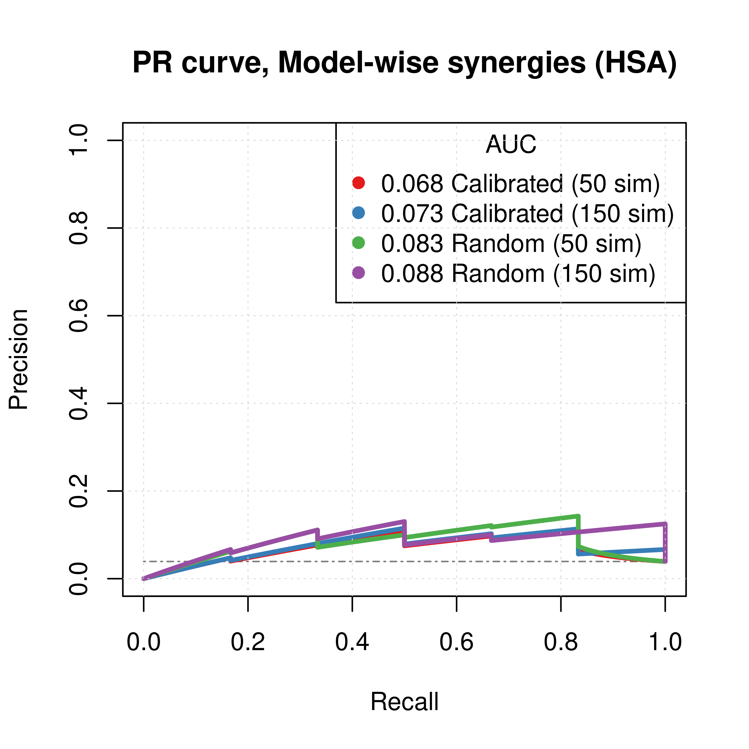
Figure 50: PR curves (CASCADE 2.0, Topology Mutations, HSA synergy method)
- The PR curves show that the performance of each individual predictor is poor compared to the baseline. Someone looking at the ROC curves only might reach a different conclusion.
- Random proliferative models perform slightly better than the calibrated ones.
- The model-wise approach produces slightly better ROC results than the ensemble-wise approach.
AUC sensitivity
Investigate same thing as described in here. This is very crucial since the PR performance is poor for the individual predictors, but a combined predictor might be able to counter this. We will combine the synergy scores from the random proliferative simulations with the results from the calibrated Gitsbe simulations (number of simulations: \(150\)).
# Ensemble-wise
betas = seq(from = -5, to = 5, by = 0.1)

prolif_roc_topo = sapply(betas, function(beta) {
  pred_topo_ew_hsa = pred_topo_ew_hsa %>% mutate(combined_score = ss_score_150sim + beta * prolif_score_150sim)
  res = roc.curve(scores.class0 = pred_topo_ew_hsa %>% pull(combined_score) %>% (function(x) {-x}),
    weights.class0 = pred_topo_ew_hsa %>% pull(observed))
  auc_value = res$auc
})

prolif_pr_topo = sapply(betas, function(beta) {
  pred_topo_ew_hsa = pred_topo_ew_hsa %>% mutate(combined_score = ss_score_150sim + beta * prolif_score_150sim)
  res = pr.curve(scores.class0 = pred_topo_ew_hsa %>% pull(combined_score) %>% (function(x) {-x}),
    weights.class0 = pred_topo_ew_hsa %>% pull(observed))
  auc_value = res$auc.davis.goadrich
})

df_ew = as_tibble(cbind(betas, prolif_roc_topo, prolif_pr_topo))
df_ew = df_ew %>% tidyr::pivot_longer(-betas, names_to = "type", values_to = "AUC")

ggline(data = df_ew, x = "betas", y = "AUC", numeric.x.axis = TRUE, color = "type",
  plot_type = "l", xlab = TeX("$\\beta$"), ylab = "AUC (Area Under Curve)",
  legend = "none", facet.by = "type", palette = my_palette, ylim = c(0,0.85),
  panel.labs = list(type = c("Precision-Recall", "ROC")),
  title = TeX("AUC sensitivity to $\\beta$ parameter")) +
  theme(plot.title = element_text(hjust = 0.5)) +
  geom_vline(xintercept = 0) +
  geom_vline(xintercept = -1, color = "black", size = 0.3, linetype = "dashed") +
  geom_text(aes(x=-1.5, label="β = -1", y=0.14), colour="black", angle=90) +
  grids()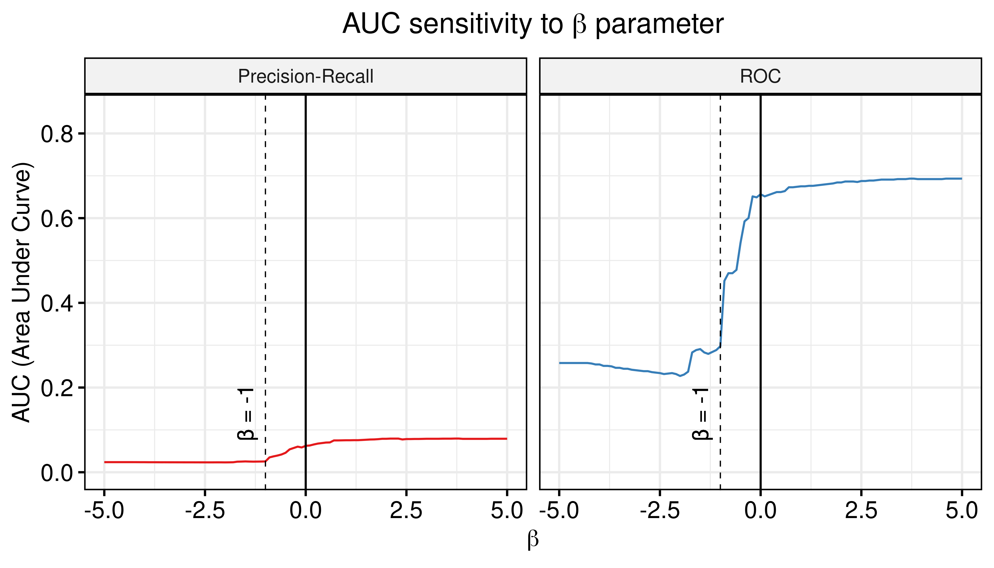
Figure 51: AUC sensitivity (CASCADE 2.0, Topology Mutations, HSA synergy method, Ensemble-wise results)
- The proliferative models do not bring any significant change to the prediction performance of the calibrated models.
Bliss Results
- Bliss refers to the synergy method used in
Drabmeto assess the synergies from thegitsbemodels - We test performance using ROC and PR AUC for both the ensemble-wise and model-wise synergies from
Drabme - Calibrated models: fitted to steady state (\(50,150\) simulations)
- Random models: fitted to proliferation profile (\(50,150\) simulations)
Gitsbemodels have only topology mutations (\(50\) mutations as a bootstrap value, \(10\) after models with stable states are found)
ROC curves
topo_res_ss_ew_50sim = get_roc_stats(df = pred_topo_ew_bliss, pred_col = "ss_score_50sim", label_col = "observed")
topo_res_ss_ew_150sim = get_roc_stats(df = pred_topo_ew_bliss, pred_col = "ss_score_150sim", label_col = "observed")
topo_res_prolif_ew_50sim = get_roc_stats(df = pred_topo_ew_bliss, pred_col = "prolif_score_50sim", label_col = "observed")
topo_res_prolif_ew_150sim = get_roc_stats(df = pred_topo_ew_bliss, pred_col = "prolif_score_150sim", label_col = "observed")

topo_res_ss_mw_50sim = get_roc_stats(df = pred_topo_mw_bliss, pred_col = "synergy_prob_ss_50sim", label_col = "observed", direction = ">")
topo_res_ss_mw_150sim = get_roc_stats(df = pred_topo_mw_bliss, pred_col = "synergy_prob_ss_150sim", label_col = "observed", direction = ">")
topo_res_prolif_mw_50sim = get_roc_stats(df = pred_topo_mw_bliss, pred_col = "synergy_prob_prolif_50sim", label_col = "observed", direction = ">")
topo_res_prolif_mw_150sim = get_roc_stats(df = pred_topo_mw_bliss, pred_col = "synergy_prob_prolif_150sim", label_col = "observed", direction = ">")

# Plot ROCs
plot(x = topo_res_ss_ew_50sim$roc_stats$FPR, y = topo_res_ss_ew_50sim$roc_stats$TPR,
  type = 'l', lwd = 3, col = my_palette[1], main = 'ROC curve, Ensemble-wise synergies (Bliss)',
  xlab = 'False Positive Rate (FPR)', ylab = 'True Positive Rate (TPR)')
lines(x = topo_res_ss_ew_150sim$roc_stats$FPR, y = topo_res_ss_ew_150sim$roc_stats$TPR,
  lwd = 3, col = my_palette[2])
lines(x = topo_res_prolif_ew_50sim$roc_stats$FPR, y = topo_res_prolif_ew_50sim$roc_stats$TPR,
  lwd = 3, col = my_palette[3])
lines(x = topo_res_prolif_ew_150sim$roc_stats$FPR, y = topo_res_prolif_ew_150sim$roc_stats$TPR,
  lwd = 3, col = my_palette[4])
legend('bottomright', title = 'AUC', col = my_palette[1:4], pch = 19,
  legend = c(paste(round(topo_res_ss_ew_50sim$AUC, digits = 2), "Calibrated (50 sim)"),
    paste(round(topo_res_ss_ew_150sim$AUC, digits = 2), "Calibrated (150 sim)"),
    paste(round(topo_res_prolif_ew_50sim$AUC, digits = 2), "Random (50 sim)"),
    paste(round(topo_res_prolif_ew_150sim$AUC, digits = 2), "Random (150 sim)")))
grid(lwd = 0.5)
abline(a = 0, b = 1, col = 'lightgrey', lty = 'dotdash', lwd = 1.2)

plot(x = topo_res_ss_mw_50sim$roc_stats$FPR, y = topo_res_ss_mw_50sim$roc_stats$TPR,
  type = 'l', lwd = 3, col = my_palette[1], main = 'ROC curve, Model-wise synergies (Bliss)',
  xlab = 'False Positive Rate (FPR)', ylab = 'True Positive Rate (TPR)')
lines(x = topo_res_ss_mw_150sim$roc_stats$FPR, y = topo_res_ss_mw_150sim$roc_stats$TPR,
  lwd = 3, col = my_palette[2])
lines(x = topo_res_prolif_mw_50sim$roc_stats$FPR, y = topo_res_prolif_mw_50sim$roc_stats$TPR,
  lwd = 3, col = my_palette[3])
lines(x = topo_res_prolif_mw_150sim$roc_stats$FPR, y = topo_res_prolif_mw_150sim$roc_stats$TPR,
  lwd = 3, col = my_palette[4])
legend('bottomright', title = 'AUC', col = my_palette[1:4], pch = 19,
  legend = c(paste(round(topo_res_ss_mw_50sim$AUC, digits = 2), "Calibrated (50 sim)"),
    paste(round(topo_res_ss_mw_150sim$AUC, digits = 2), "Calibrated (150 sim)"),
    paste(round(topo_res_prolif_mw_50sim$AUC, digits = 2), "Random (50 sim)"),
    paste(round(topo_res_prolif_mw_150sim$AUC, digits = 2), "Random (150 sim)")))
grid(lwd = 0.5)
abline(a = 0, b = 1, col = 'lightgrey', lty = 'dotdash', lwd = 1.2)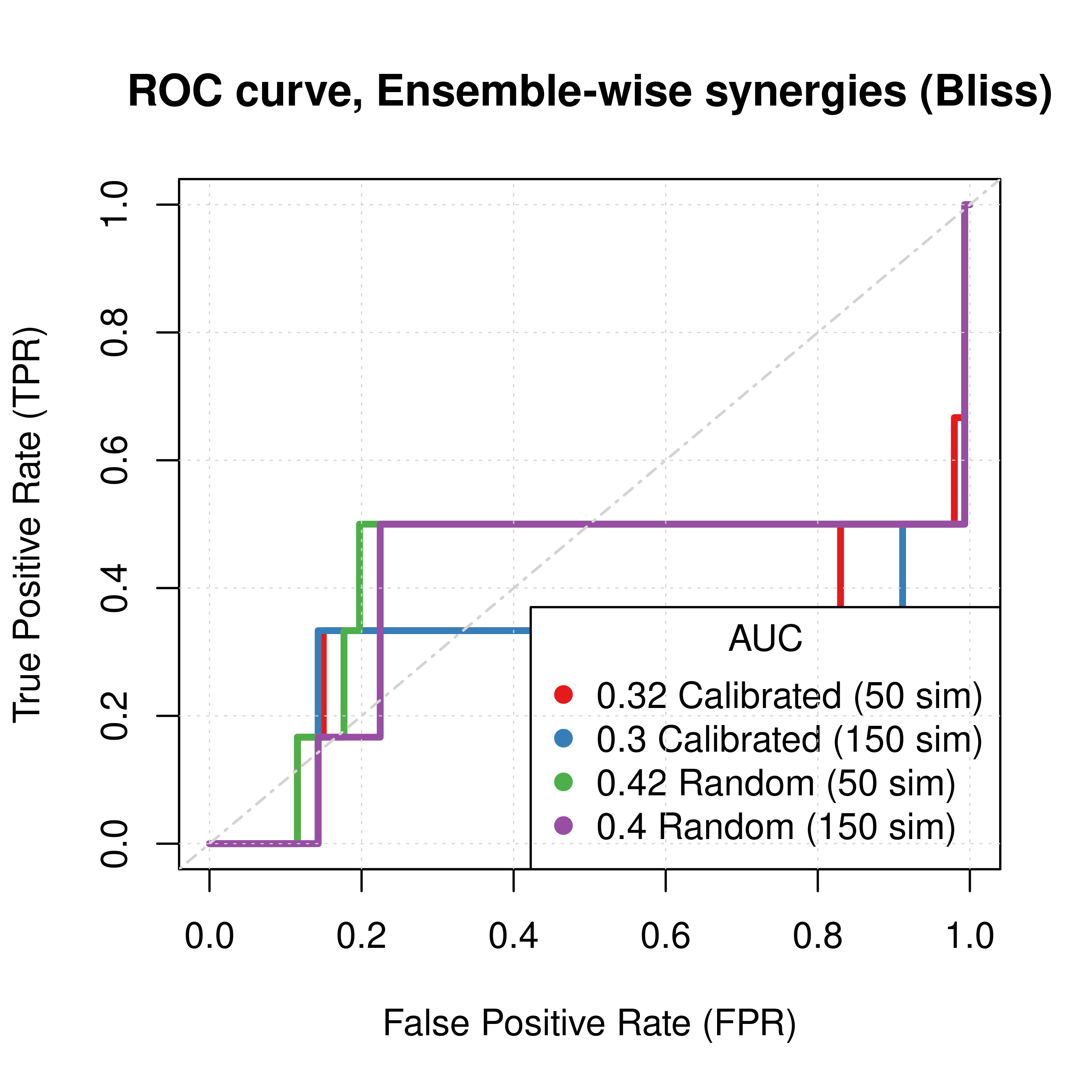
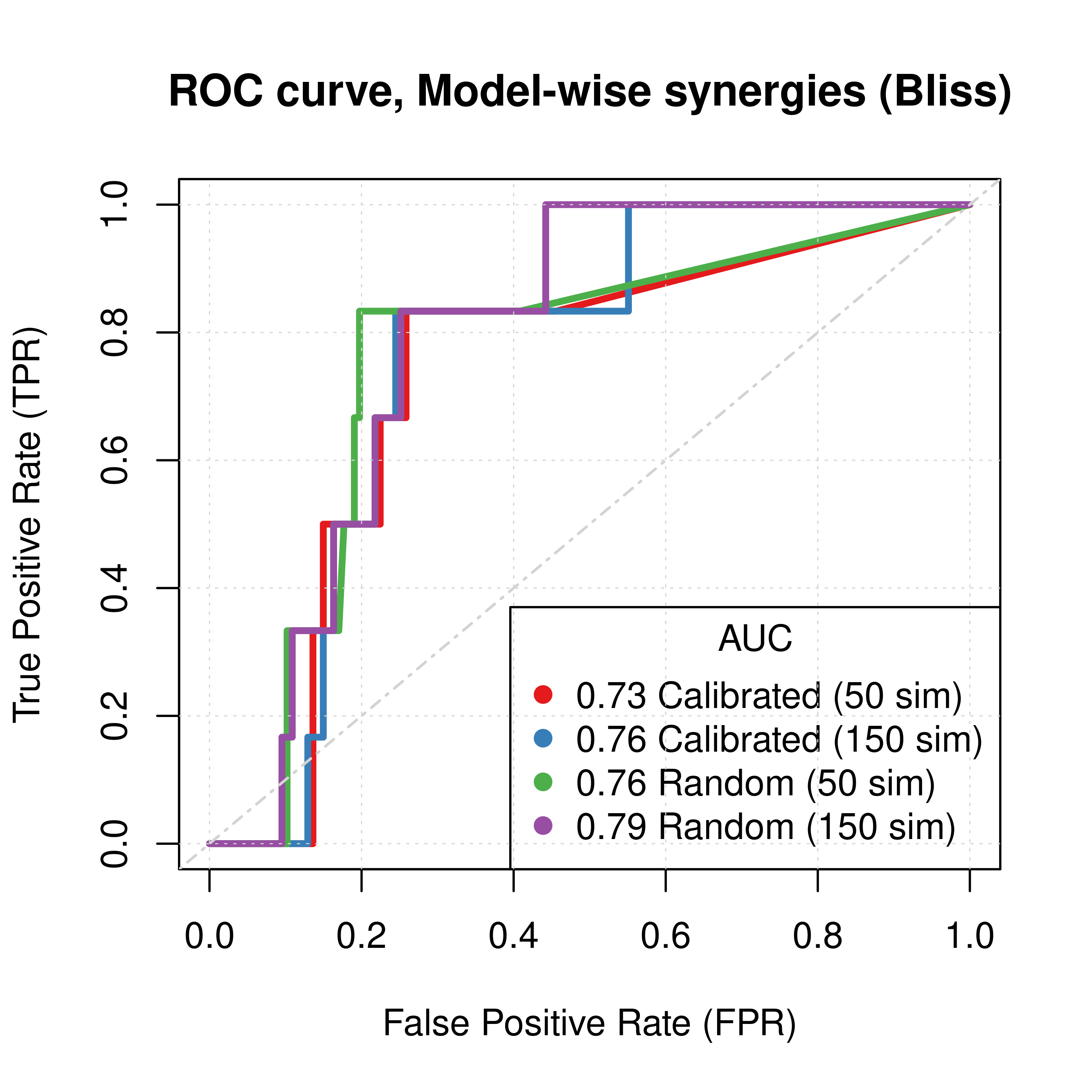
Figure 52: ROC curves (CASCADE 2.0, Topology Mutations, Bliss synergy method)
PR curves
pr_topo_res_ss_ew_50sim = pr.curve(scores.class0 = pred_topo_ew_bliss %>% pull(ss_score_50sim) %>% (function(x) {-x}),
  weights.class0 = pred_topo_ew_bliss %>% pull(observed), curve = TRUE, rand.compute = TRUE)
pr_topo_res_ss_ew_150sim = pr.curve(scores.class0 = pred_topo_ew_bliss %>% pull(ss_score_150sim) %>% (function(x) {-x}),
  weights.class0 = pred_topo_ew_bliss %>% pull(observed), curve = TRUE)
pr_topo_res_prolif_ew_50sim = pr.curve(scores.class0 = pred_topo_ew_bliss %>% pull(prolif_score_50sim) %>% (function(x) {-x}),
  weights.class0 = pred_topo_ew_bliss %>% pull(observed), curve = TRUE)
pr_topo_res_prolif_ew_150sim = pr.curve(scores.class0 = pred_topo_ew_bliss %>% pull(prolif_score_150sim) %>% (function(x) {-x}),
  weights.class0 = pred_topo_ew_bliss %>% pull(observed), curve = TRUE)

pr_topo_res_ss_mw_50sim = pr.curve(scores.class0 = pred_topo_mw_bliss %>% pull(synergy_prob_ss_50sim),
  weights.class0 = pred_topo_mw_bliss %>% pull(observed), curve = TRUE, rand.compute = TRUE)
pr_topo_res_ss_mw_150sim = pr.curve(scores.class0 = pred_topo_mw_bliss %>% pull(synergy_prob_ss_150sim),
  weights.class0 = pred_topo_mw_bliss %>% pull(observed), curve = TRUE)
pr_topo_res_prolif_mw_50sim = pr.curve(scores.class0 = pred_topo_mw_bliss %>% pull(synergy_prob_prolif_50sim),
  weights.class0 = pred_topo_mw_bliss %>% pull(observed), curve = TRUE)
pr_topo_res_prolif_mw_150sim = pr.curve(scores.class0 = pred_topo_mw_bliss %>% pull(synergy_prob_prolif_150sim),
  weights.class0 = pred_topo_mw_bliss %>% pull(observed), curve = TRUE)

plot(pr_topo_res_ss_ew_50sim, main = 'PR curve, Ensemble-wise synergies (Bliss)',
  auc.main = FALSE, color = my_palette[1], rand.plot = TRUE)
plot(pr_topo_res_ss_ew_150sim, add = TRUE, color = my_palette[2])
plot(pr_topo_res_prolif_ew_50sim, add = TRUE, color = my_palette[3])
plot(pr_topo_res_prolif_ew_150sim, add = TRUE, color = my_palette[4])
legend('topright', title = 'AUC', col = my_palette[1:4], pch = 19,
  legend = c(paste(round(pr_topo_res_ss_ew_50sim$auc.davis.goadrich, digits = 3), "Calibrated (50 sim)"),
    paste(round(pr_topo_res_ss_ew_150sim$auc.davis.goadrich, digits = 3), "Calibrated (150 sim)"),
    paste(round(pr_topo_res_prolif_ew_50sim$auc.davis.goadrich, digits = 3), "Random (50 sim)"),
    paste(round(pr_topo_res_prolif_ew_150sim$auc.davis.goadrich, digits = 3), "Random (150 sim)")))
grid(lwd = 0.5)

plot(pr_topo_res_ss_mw_50sim, main = 'PR curve, Model-wise synergies (Bliss)',
  auc.main = FALSE, color = my_palette[1], rand.plot = TRUE)
plot(pr_topo_res_ss_mw_150sim, add = TRUE, color = my_palette[2])
plot(pr_topo_res_prolif_mw_50sim, add = TRUE, color = my_palette[3])
plot(pr_topo_res_prolif_mw_150sim, add = TRUE, color = my_palette[4])
legend('topright', title = 'AUC', col = my_palette[1:4], pch = 19,
  legend = c(paste(round(pr_topo_res_ss_mw_50sim$auc.davis.goadrich, digits = 3), "Calibrated (50 sim)"),
    paste(round(pr_topo_res_ss_mw_150sim$auc.davis.goadrich, digits = 3), "Calibrated (150 sim)"),
    paste(round(pr_topo_res_prolif_mw_50sim$auc.davis.goadrich, digits = 3), "Random (50 sim)"),
    paste(round(pr_topo_res_prolif_mw_150sim$auc.davis.goadrich, digits = 3), "Random (150 sim)")))
grid(lwd = 0.5)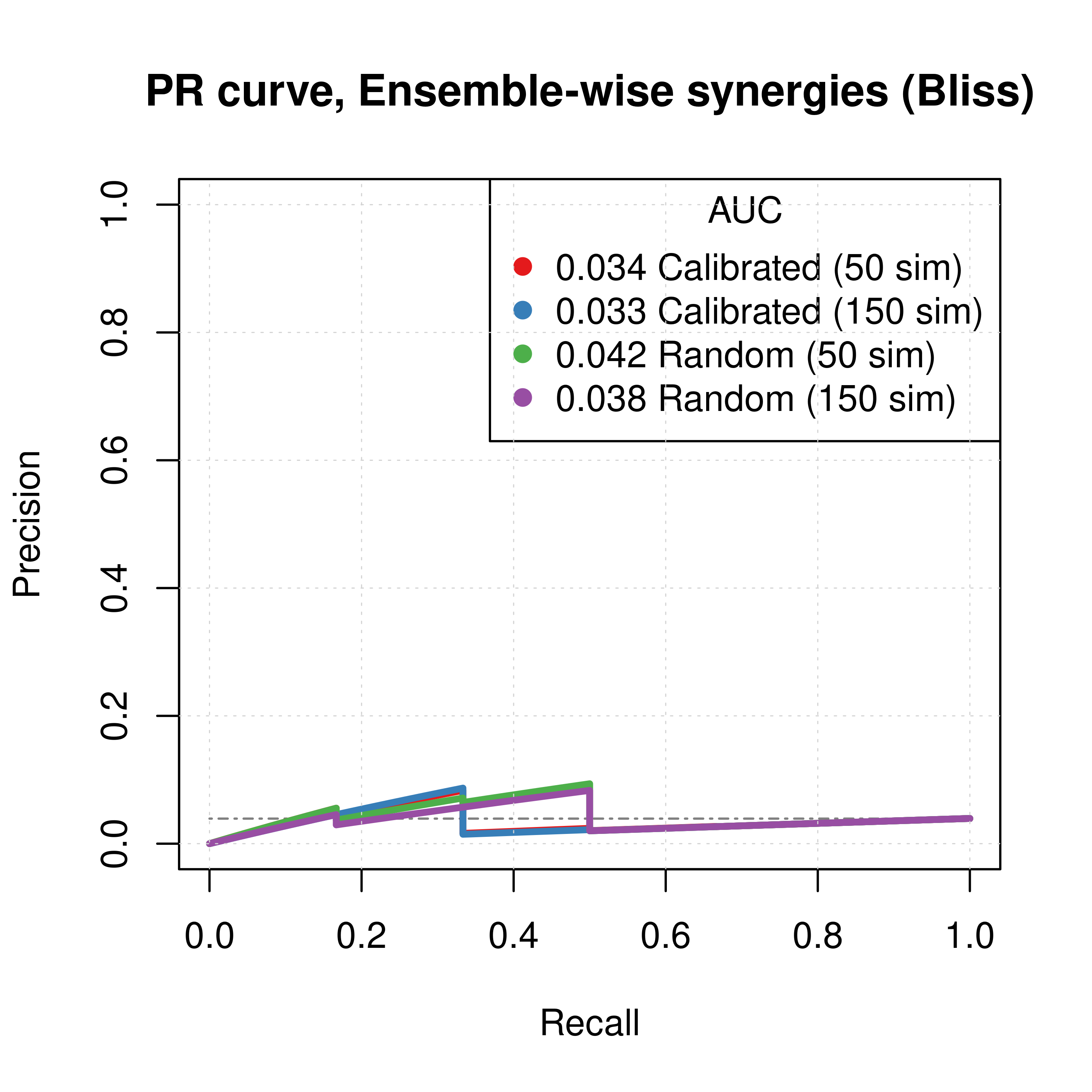
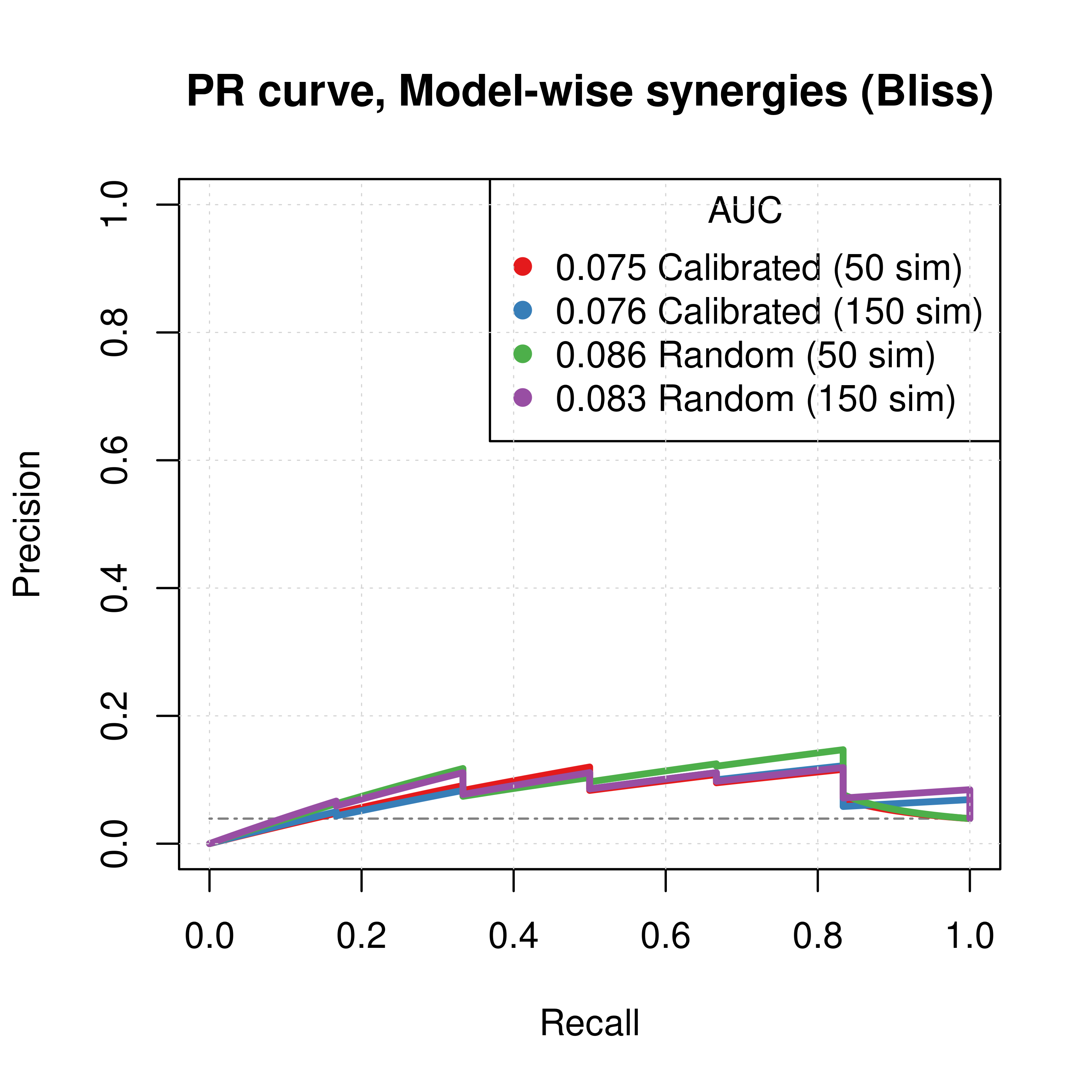
Figure 53: PR curves (CASCADE 2.0, Topology Mutations, Bliss synergy method)
- The PR curves show that the performance of all individual predictors is poor compared to the baseline.
- Random proliferative models perform slightly better than the calibrated ones.
- The model-wise approach produces slightly better ROC and PR results than the ensemble-wise approach
AUC sensitivity
Investigate same thing as described in here. This is very crucial since the PR performance is poor for the individual predictors, but a combined predictor might be able to counter this. We will combine the synergy scores from the random proliferative simulations with the results from the calibrated Gitsbe simulations (number of simulations: \(150\)).
# Ensemble-wise
betas = seq(from = -5, to = 5, by = 0.1)

prolif_roc = sapply(betas, function(beta) {
  pred_topo_ew_bliss = pred_topo_ew_bliss %>% mutate(combined_score = ss_score_150sim + beta * prolif_score_150sim)
  res = roc.curve(scores.class0 = pred_topo_ew_bliss %>% pull(combined_score) %>% (function(x) {-x}),
    weights.class0 = pred_topo_ew_bliss %>% pull(observed))
  auc_value = res$auc
})

prolif_pr = sapply(betas, function(beta) {
  pred_topo_ew_bliss = pred_topo_ew_bliss %>% mutate(combined_score = ss_score_150sim + beta * prolif_score_150sim)
  res = pr.curve(scores.class0 = pred_topo_ew_bliss %>% pull(combined_score) %>% (function(x) {-x}),
    weights.class0 = pred_topo_ew_bliss %>% pull(observed))
  auc_value = res$auc.davis.goadrich
})

df_ew = as_tibble(cbind(betas, prolif_roc, prolif_pr))
df_ew = df_ew %>% tidyr::pivot_longer(-betas, names_to = "type", values_to = "AUC")

ggline(data = df_ew, x = "betas", y = "AUC", numeric.x.axis = TRUE, color = "type",
  plot_type = "l", xlab = TeX("$\\beta$"), ylab = "AUC (Area Under Curve)",
  legend = "none", facet.by = "type", palette = my_palette, ylim = c(0,0.85),
  panel.labs = list(type = c("Precision-Recall", "ROC")),
  title = TeX("AUC sensitivity to $\\beta$ parameter")) +
  theme(plot.title = element_text(hjust = 0.5)) +
  geom_vline(xintercept = 0) +
  geom_vline(xintercept = -1, color = "black", size = 0.3, linetype = "dashed") +
  geom_text(aes(x=-1.5, label="β = -1", y=0.15), colour="black", angle = 90) +
  grids()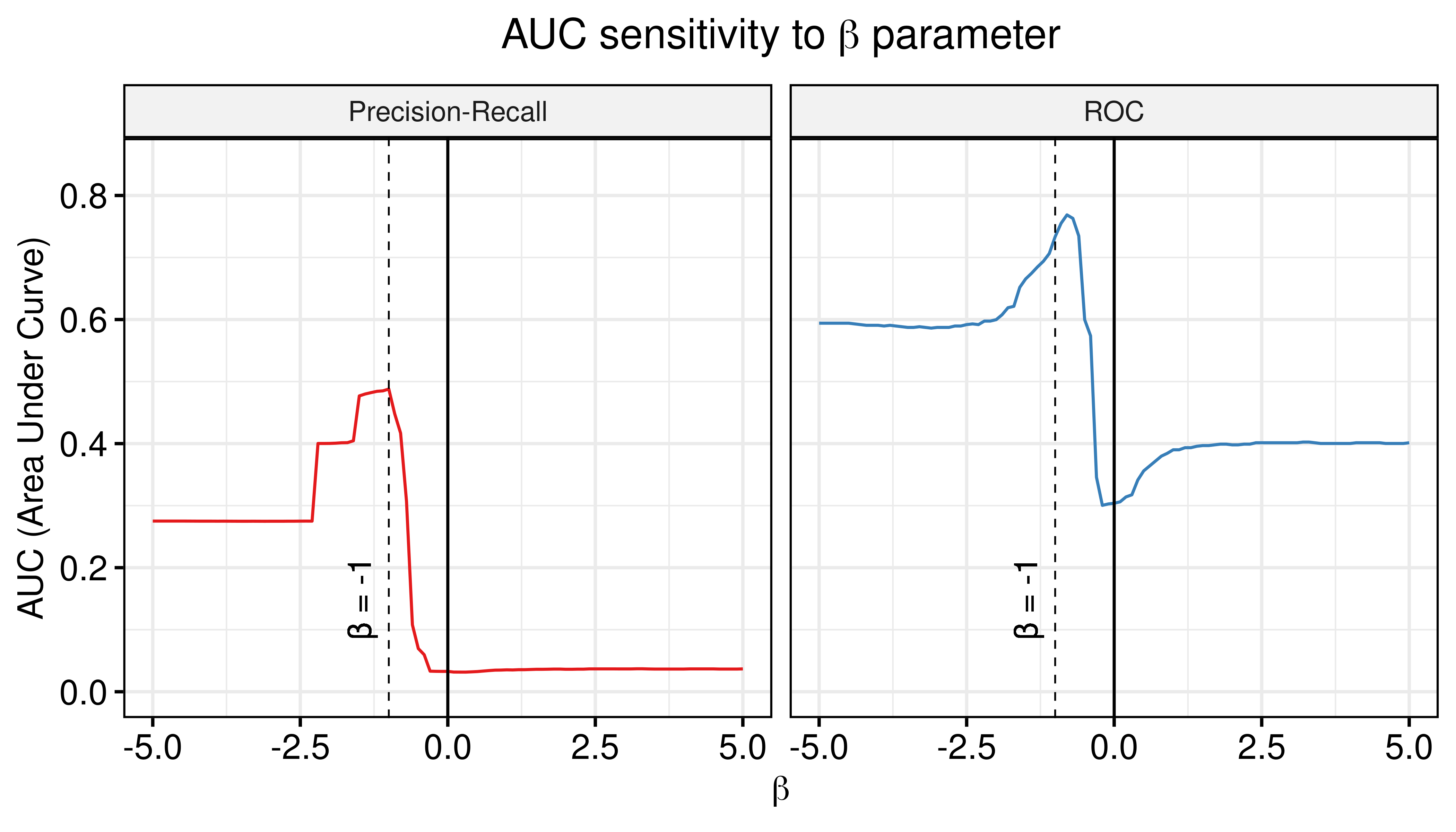
Figure 54: AUC sensitivity (CASCADE 2.0, Topology Mutations, Bliss synergy method, Ensemble-wise results)
- The proliferative models can be used to normalize against the predictions of the calibrated models and thus bring significant contribution to the calibrated models performance (both ROC-AUC and PR-AUC are increased).
- The \(\beta_{best}\) values of the combined calibrated and random proliferative model predictor that maximize the ROC-AUC and PR-AUC respectively are \(\beta_{best}^{\text{ROC-AUC}}=-0.8\) and \(\beta_{best}^{\text{PR-AUC}}=-1\)
Best ROC and PRC
For the Bliss ensemble-wise results we demonstrated above that a value of \(\beta_{best}=-1\) can result in significant performance gain of the combined predictor (\(calibrated + \beta \times random\)). So, the best ROC and PR curves we can get with our simulations when using models with topology mutations are:
best_beta = -1
pred_topo_ew_bliss = pred_topo_ew_bliss %>% mutate(best_score = ss_score_150sim + best_beta * prolif_score_150sim)

roc_best_res = get_roc_stats(df = pred_topo_ew_bliss, pred_col = "best_score", label_col = "observed")
pr_best_res = pr.curve(scores.class0 = pred_topo_ew_bliss %>% pull(best_score) %>% (function(x) {-x}),
    weights.class0 = pred_topo_ew_bliss %>% pull(observed), curve = TRUE, rand.compute = TRUE)

# Plot best ROC
plot(x = roc_best_res$roc_stats$FPR, y = roc_best_res$roc_stats$TPR,
  type = 'l', lwd = 3, col = my_palette[1], main = TeX('ROC curve (Ensemble-wise), $calibrated + \\beta \\times random$'),
  xlab = 'False Positive Rate (FPR)', ylab = 'True Positive Rate (TPR)')
legend('bottomright', title = TeX('AUC ($\\beta$ = -1)'), col = my_palette[1], pch = 19,
  legend = paste(round(roc_best_res$AUC, digits = 2), 'Bliss (150 sim)'), cex = 1.5)
grid(lwd = 0.5)
abline(a = 0, b = 1, col = 'lightgrey', lty = 'dotdash', lwd = 1.2)

# Plot best PRC
plot(pr_best_res, main = TeX('PR curve (Ensemble-wise), $calibrated + \\beta \\times random$'),
  auc.main = FALSE, color = my_palette[2], rand.plot = TRUE)
legend('topright', title = TeX('AUC ($\\beta$ = -1)'), col = my_palette[2], pch = 19,
  legend = paste(round(pr_best_res$auc.davis.goadrich, digits = 2), 'Bliss (150 sim)'), cex = 1.5)
grid(lwd = 0.5)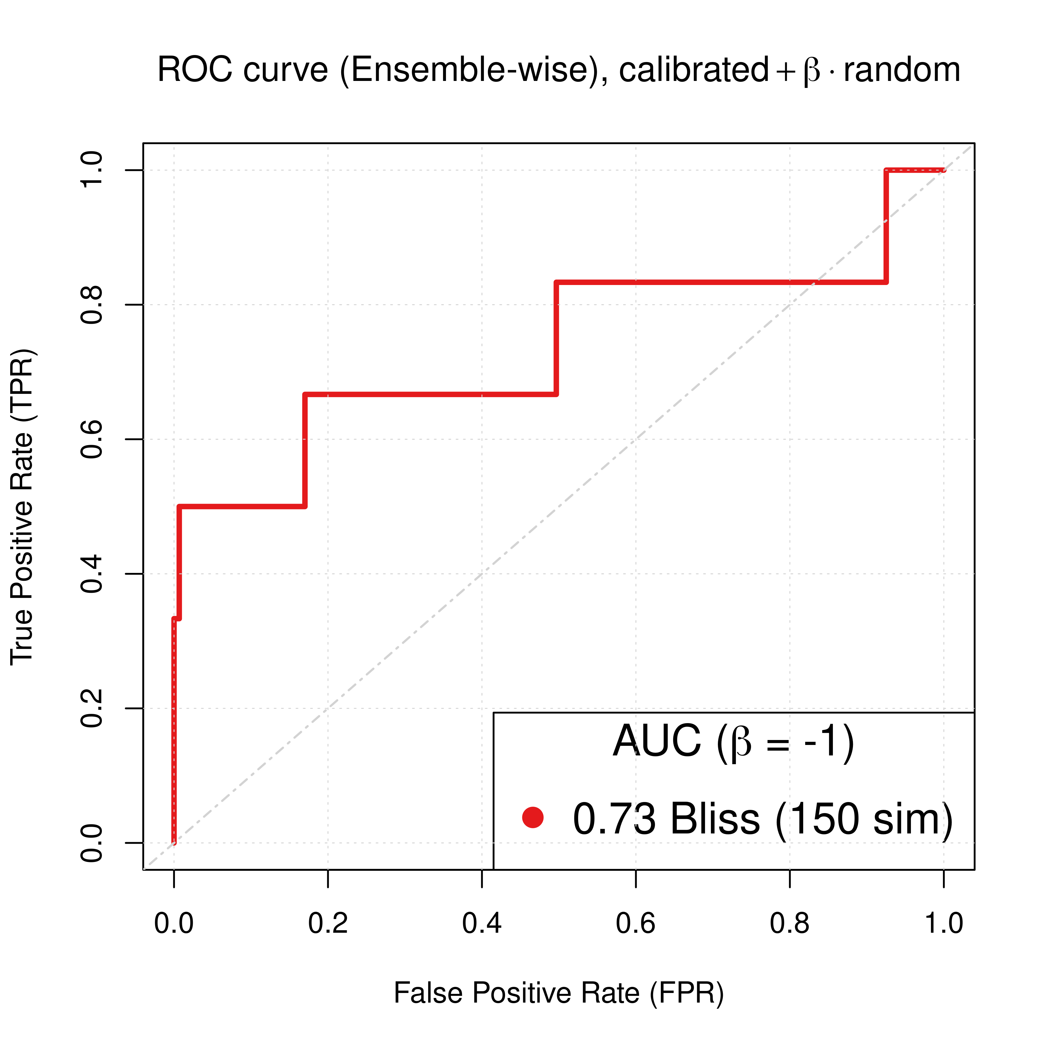
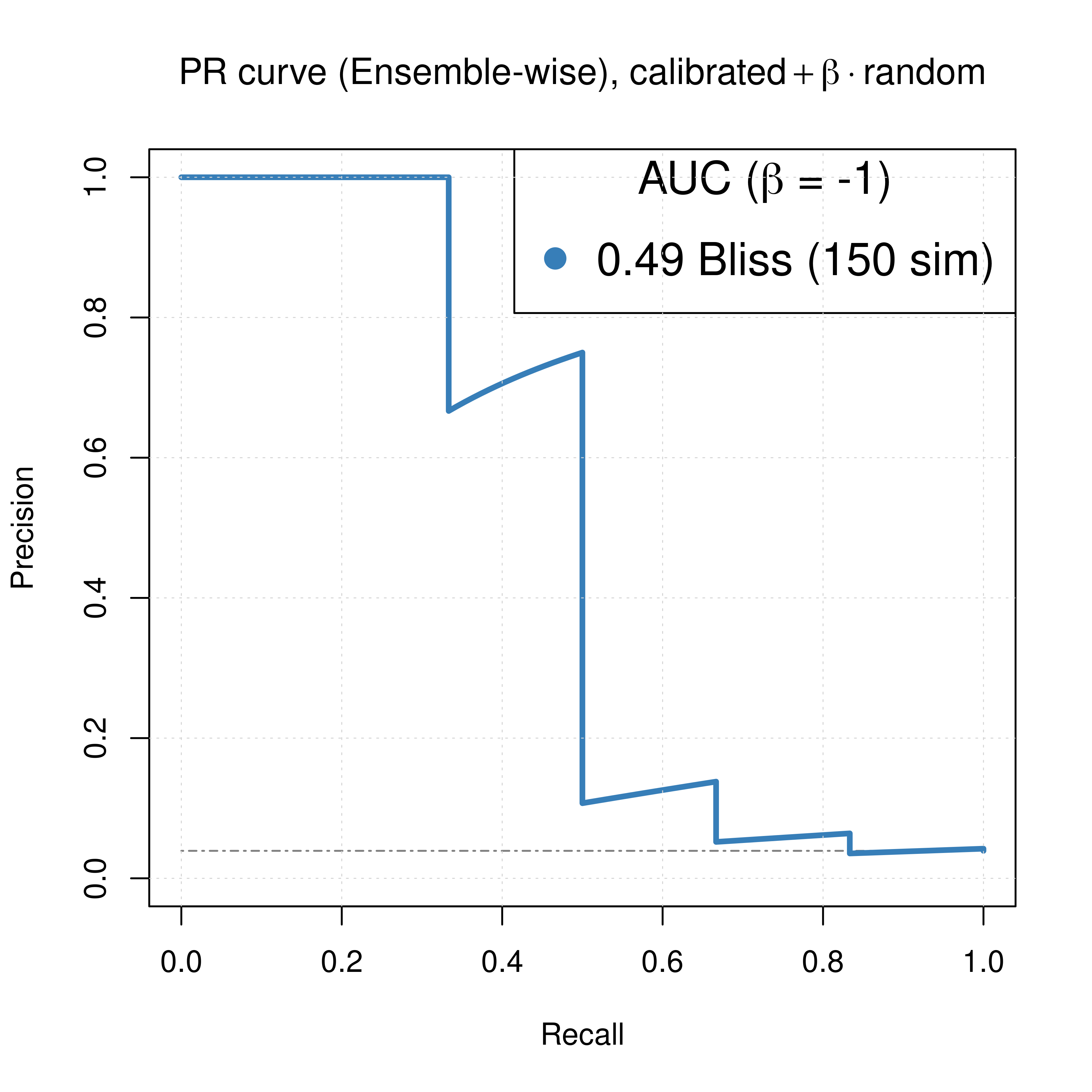
Figure 55: ROC and PR curve for best beta (CASCADE 2.0, Topology Mutations)
Fitness vs Ensemble Performance
We check for correlation between the calibrated models fitness to the AGS steady state and their ensemble performance subject to normalization to the random model predictions.
The main idea here is that we generate different training data samples, in which the boolean steady state nodes have their values flipped (so they are only partially correct) and we fit models to these (\(50\) simulations => \(150\) topology-mutated models per training data, \(205\) training data samples in total). These calibrated model ensembles can then be tested for their prediction performance. Then we use the ensemble-wise random proliferative model predictions (\(50\) simulations) to normalize (\(\beta=-1\)) against the calibrated model predictions and compute the AUC ROC and AUC PR for each model ensemble.
Check how to generate the appropriate data, run the simulations and tidy up the results in the section Fitness vs Performance Methods.
Load the already-stored result:
res = readRDS(file = "data/res_fit_aucs_topo.rds")We check if our data is normally distributed using the Shapiro-Wilk normality test:
shapiro.test(x = res$roc_auc)
    Shapiro-Wilk normality test

data:  res$roc_auc
W = 0.98463, p-value = 0.02488shapiro.test(x = res$pr_auc)
    Shapiro-Wilk normality test

data:  res$pr_auc
W = 0.92214, p-value = 6.025e-09shapiro.test(x = res$avg_fit)
    Shapiro-Wilk normality test

data:  res$avg_fit
W = 0.88305, p-value = 1.609e-11
We observe from the low p-values that the data is not normally distributed. Thus, we are going to use a non-parametric correlation metric, namely the Kendall rank-based test (and it’s respective coefficient, \(\tau\)), to check for correlation between the ensemble model performance (ROC-AUC, PR-AUC) and the fitness to the AGS steady state:
p = ggpubr::ggscatter(data = res, x = "avg_fit", y = "roc_auc", color = "per_flipped_data",
  xlab = "Average Fitness per Model Ensemble",
  title = "Fitness to AGS Steady State vs Performance (ROC)",
  ylab = "ROC AUC", add = "reg.line", conf.int = TRUE,
  add.params = list(color = "blue", fill = "lightgray"),
  cor.coef = TRUE, cor.coeff.args = list(method = "kendall", size = 6, cor.coef.name = "tau")) +
  theme(plot.title = element_text(hjust = 0.5)) +
  scale_color_distiller(n.breaks = 5, labels = scales::label_percent(accuracy = 1L), palette = 'RdYlBu', guide = guide_colourbar(title = '%Data Flipped'))
ggpubr::ggpar(p, legend = "right", font.legend = 14)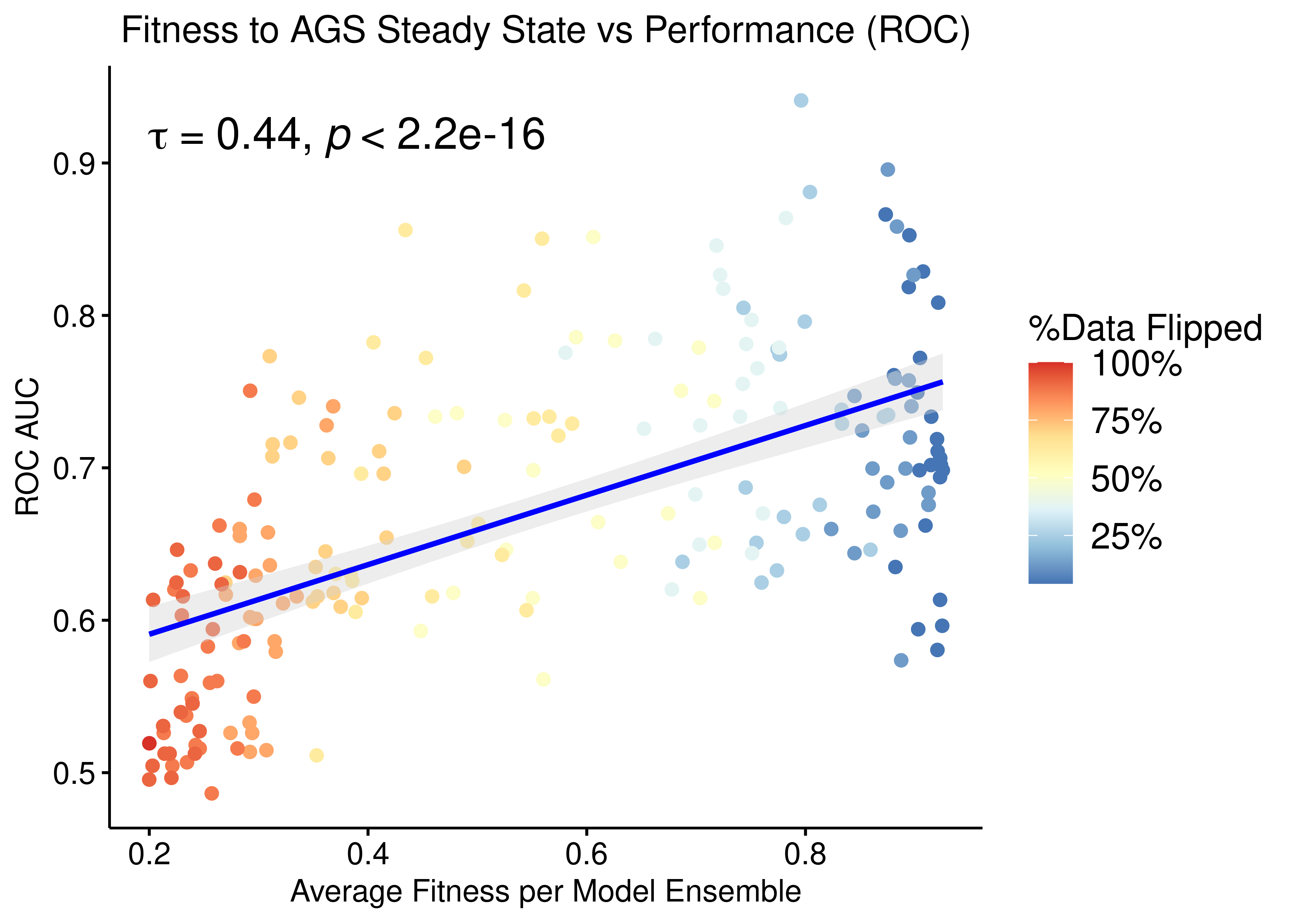
Figure 56: Fitness to AGS Steady State vs ROC-AUC Performance (CASCADE 2.0, Topology mutations, Bliss synergy method, Ensemble-wise normalized results)
p = ggpubr::ggscatter(data = res, x = "avg_fit", y = "pr_auc", color = "per_flipped_data",
  xlab = "Average Fitness per Model Ensemble",
  title = "Fitness to AGS Steady State vs Performance (Precision-Recall)",
  add.params = list(color = "blue", fill = "lightgray"),
  ylab = "PR AUC", add = "reg.line", conf.int = TRUE,
  cor.coef = TRUE, cor.coeff.args = list(method = "kendall", size = 6, cor.coef.name = "tau")) +
  theme(plot.title = element_text(hjust = 0.5)) +
  scale_color_distiller(n.breaks = 5, labels = scales::label_percent(accuracy = 1L), palette = 'RdYlBu', guide = guide_colourbar(title = '%Data Flipped'))
ggpubr::ggpar(p, legend = "right", font.legend = 14)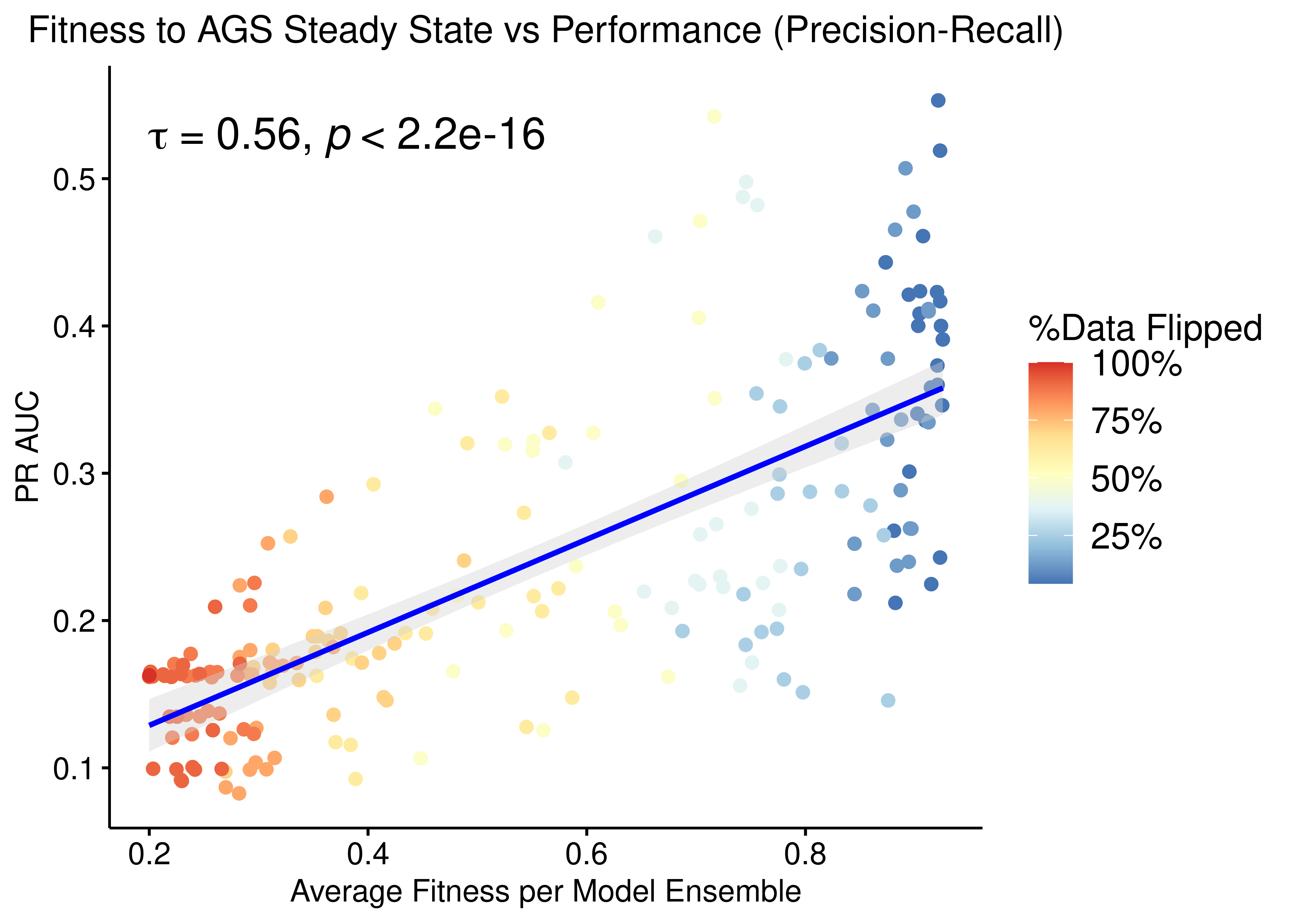
Figure 57: Fitness to AGS Steady State vs PR-AUC Performance (CASCADE 2.0, Topology Mutations, Bliss synergy method, Ensemble-wise normalized results)
- We observe that there exists some correlation between the normalized ensemble model performance vs the models fitness to the training steady state data.
- Correlation results are better than when applying link-operator mutations to the models. The topology mutations offer a larger variation in performance in terms of both ROC and PR AUC, given the limited set of provided steady state nodes for calibration of the models (24 out of 144 in total for the AGS cell line).
- The performance as measured by the ROC AUC is less sensitive to changes in the training data but there is better correlation with regards to the PR AUC, which is a more informative measure for our imbalanced dataset (Saito and Rehmsmeier 2015).