Truth Density Data Analysis

Data

I created every possible truth table for up to \(20\) variables (variables here means regulators for us) and calculated the “AND-NOT”, “OR-NOT”, “Pairs”, “Act-win”, “Inh-win” Boolean function results for every possible configuration of the number of activators and inhibitors that added up to the number of regulators. Then, from the truth tables I calculated the truth density of each function for each particular configuration. For more details see the script get_stats.R

See the data below:

stats = readRDS(file = "data/td_stats.rds")

DT::datatable(data = stats,
  caption = htmltools::tags$caption("Truth Density Data", style="color:#dd4814; font-size: 18px"),
  options = list(pageLength = 6, scrollX = TRUE, order = list(list(1, "asc")))) %>% 
  formatRound(4:8, digits = 2)

Truth Density formulas

In this section we prove the exact formulas for the truth densities in the case of the \(f_{AND-NOT}\), \(f_{OR-NOT}\) and \(f_{Pairs}\) link operator Boolean functions, as well as for the two threshold functions \(f_{Act-win}\) and \(f_{Inh-win}\). We also show how each truth density formula asymptotically behaves for a large number of regulators and investigate the cases where there is either balance or imbalance between the number of activators and inhibitors. Lastly, we validate the proofs with the above data.

TD Proofs

For all propositions presented, we assume that:

1. \(f\) is a Boolean function \(f(x,y):\{0,1\}^n \rightarrow \{0,1\}\), with a total of \(n\) regulators/input variables
2. The regulators are uniquely separated to two distinct groups: \(m\) activators (positive regulators) \(x=\{x_i\}_{i=1}^{m}\) and \(k\) inhibitors (negative regulators) \(y=\{y_j\}_{j=1}^{k}\), with \(n = m + k\) and \(m,k \ge 1\).

Proposition 1 (AND-NOT Truth Density Formula) When a Boolean regulatory function \(f\) has the form of an AND-NOT link operator Boolean function: \(f_{AND-NOT}(x,y) = \left(\bigvee_{i=1}^{m} x_i\right) \land \lnot \left(\bigvee_{j=1}^{k} y_j\right)\) with \(m \ge 1\) activators and \(k \ge 1\) inhibitors, its truth density is \(TD_{AND-NOT}=\frac{2^m-1}{2^n} = \frac{1}{2^k}-\frac{1}{2^n}\).

Proof. Using the distributivity property and De Morgan’s law we can re-write \(f_{AND-NOT}\) in a DNF form as: \[\begin{equation} \begin{split} f_{AND-NOT}(x,y) & = \left(\bigvee_{i=1}^{m} x_i\right) \land \lnot \left(\bigvee_{j=1}^{k} y_j\right) \\ & = \bigvee_{i=1}^{m} \left( x_i \land \lnot \left( \bigvee_{j=1}^{k} y_j \right) \right) \\ & = \bigvee_{i=1}^{m} (x_i \land \bigwedge_{j=1}^{k} \lnot y_j) \\ & = \bigvee_{i=1}^{m} (x_i \land \lnot y_1 \land ... \land \lnot y_k) \end{split} \end{equation}\]

To calculate the \(TD_{AND-NOT}\), we need to find the number of rows of the \(f_{AND-NOT}\) truth table that result in a TRUE output result and divide that by the total number of rows, which is \(2^n\) (\(n\) regulators/inputs). Note that \(f_{AND-NOT}\), written in it’s equivalent DNF form, has exactly \(m\) terms. Each term has a unique TRUE/FALSE assignment of regulators that makes it TRUE. This happens when the activator of the term is TRUE and all of the inhibitors FALSE. Since the condition for the inhibitors is the same regardless of the term we are looking at and \(f\) is expressed in a DNF form, the TRUE outcomes of the function \(f\) are defined by all logical assignment combinations of the \(m\) activators that have at least one of them being TRUE and all inhibitors assigned as FALSE. There are a total of \(2^m\) possible \(TRUE/FALSE\) logical assignments of the \(m\) activators (from all FALSE to all TRUE) and \(f_{AND-NOT}\) becomes TRUE on all except one of them (i.e. when all activators are FALSE) and the corresponding \(2^m-1\) truth table rows have all inhibitors assigned as FALSE. Thus \(TD_{AND-NOT}=\frac{2^m-1}{2^n}\).

Proposition 2 (OR-NOT Truth Density Formula) When a Boolean regulatory function \(f\) has the form of an OR-NOT link operator Boolean function: \(f_{OR-NOT}(x,y) = \left(\bigvee_{i=1}^{m} x_i\right) \lor \lnot \left(\bigvee_{j=1}^{k} y_j\right)\) with \(m \ge 1\) activators and \(k \ge 1\) inhibitors, its truth density is \(TD_{OR-NOT}=\frac{2^n-(2^k-1)}{2^n} = 1 + \frac{1}{2^n} - \frac{1}{2^m}\).

Proof. Using De Morgan’s law we can re-write \(f_{OR-NOT}\) in a DNF form as: \[\begin{equation} \begin{split} f_{OR-NOT}(x,y) & = \left(\bigvee_{i=1}^{m} x_i\right) \lor \lnot \left(\bigvee_{j=1}^{k} y_j\right) \\ & = \left(\bigvee_{i=1}^{m} x_i\right) \lor \left(\bigwedge_{j=1}^{k} \lnot y_j\right) \\ & = x_1 \lor x_2 \lor ... \lor x_m \lor (\lnot y_1 \land ... \land \lnot y_k) \end{split} \end{equation}\]

To calculate the \(TD_{OR-NOT}\), we find the number of rows of the \(f_{OR-NOT}\) truth table that result in a FALSE output result (\(R_{false}\)), subtract that number from the total number of rows (\(2^n\)) to get the rows that result in \(f\) being TRUE and then divide by the total number of rows. Thus \(TD_{OR-NOT} = \frac{2^n-R_{false}}{2^n}\). Note that \(f_{OR-NOT}\), written in it’s equivalent DNF form, has exactly \(m+1\) terms. To make \(f_{OR-NOT}\) FALSE, we first need to assign the \(m\) activators as FALSE and then it all depends on the logical assignments of the inhibitors \(y_j\) that are part of the last DNF term. Out of all possible \(2^k\) TRUE/FALSE logical assignments of the \(k\) inhibitors (ranging from all FALSE to all TRUE) there is only one that does not make the last term of \(f_{OR-NOT}\) FALSE (i.e. it makes the term TRUE) and that happens when all \(k\) inhibitors are FALSE. Thus, \(R_{false}=2^k-1\) and \(TD_{OR-NOT}=\frac{2^n-(2^k-1)}{2^n}\).

Proposition 3 (Pairs Truth Density Formula) When a Boolean regulatory function \(f\) has the form of a Pairs link operator Boolean function: \(f_{Pairs}(x,y) = \left(\bigvee_{i=1}^{m} x_i\right) \land \left(\bigvee_{j=1}^{k} \lnot y_j\right)\) with \(m \ge 1\) activators and \(k \ge 1\) inhibitors, its truth density is \(TD_{Pairs}=\frac{2^n-2^k-2^m+1}{2^n} = 1 - \frac{2^k+2^m-1}{2^n}\).

Proof. To calculate the \(TD_{Pairs}\) based on its given CNF, we find the number of rows in its truth table that have at least one present/TRUE activator (\(R_{act}\)) and subtract from these the rows in which all inhibitors are present/TRUE (\(R_{inh}\)). Thus only the rows that have at least one inhibitor absent/FALSE will be left (and of course at least one activator present), which corresponds exactly to the \(f_{Pairs}\) formula’s biological interpretation.

\(R_{act}\) can be found by subtracting from the total number of rows (\(2^n\)) the rows that have all activators absent/FALSE. How many are these rows? Their number depends on the number of inhibitors, since for each one of the total possible \(2^k\) TRUE/FALSE logical assignments of the \(k\) inhibitors (ranging from all FALSE to all TRUE), there will be a row in the truth table with all activators as FALSE. Thus, \(R_{act} = 2^n - 2^k\).

\(R_{inh}\) depends on the number of activators, since for each one of the total possible \(2^m\) TRUE/FALSE assignments of the \(m\) activators (ranging from all FALSE to all TRUE), there will be a row in the truth table with all inhibitors as TRUE. Note that we have to exclude one row from this result, exactly the row that has all activators as FALSE since it’s not included in the \(R_{act}\) rows. Thus, \(R_{inh}=2^m-1\) and \(TD_{Pairs}=\frac{R_{act}-R_{inh}}{2^n}=\frac{2^n-2^k-2^m+1}{2^n}\).

Proposition 4 (Threshold Functions Truth Density Formulas) When a Boolean regulatory function \(f\) has the form of either a “Act-win” or a “Inh-win” threshold function:

\[f_{Act-win}(x,y)=\begin{cases} 1, & \text{for } \sum_{i=1}^{m} x_i \ge \sum_{j=1}^{k} y_j\\ 0, & \text{otherwise} \end{cases}\]

\[f_{Inh-win}(x,y)=\begin{cases} 1, & \text{for } \sum_{i=1}^{m} x_i \gt \sum_{j=1}^{k} y_j\\ 0, & \text{otherwise} \end{cases}\]

, its respective truth density is given by the formulas:

\[TD_{Act-win}=\frac{\sum_{i=1}^m \left[ \binom{m}{i} \sum_{j=0}^{min(i,k)} \binom{k}{j} \right]}{2^n}\]

and

\[TD_{Inh-win}=\frac{\sum_{i=1}^m \left[ \binom{m}{i} \sum_{j=0}^{min(i-1,k)} \binom{k}{j} \right]}{2^n}\]

Proof. The above formulas are easily derived from the observation that we need to count the number of rows in the respective truth tables that have more present (assigned to TRUE) activators than present inhibitors (or equal in the case of \(f_{Act-win}\) but that’s a detail as we will see).

Firstly, we count all the subset input configurations that have up to \(m\) activators present. These include the partial TRUE/FALSE assignments that have just a single activator present, a pair of activators present, a triplet, etc. This is exactly the term \(\sum_{i=1}^m \binom{m}{i}\). Note that each of these activator input configurations is multiplied by a factor of \(2^k\) in the truth table to make ‘full’ rows, where the activator values stay the same and the inhibitor values range from all FALSE to all TRUE. Thus, we need to specify exactly which inhibitor assignments are appropriate for each activator subset input configuration. To do that, we multiply the size of each activator subset \(\binom{m}{i}\) with the number of configurations that have less inhibitors present, i.e. \(\sum_{j=0}^{i-1} \binom{k}{j}\).

For example, if we take the number of subsets with \(i=2\) activators present \(\binom{m}{2}\), we need to multiply by the number of configurations that have one or no present inhibitors \(\sum_{j=0}^{1} \binom{k}{j}\) to find the number of rows of interest. That is of course the case of the \(f_{Inh-win}\) function. For the \(f_{Act-win}\), we would have to add up to the present inhibitor pairs: \(\sum_{j=0}^{2} \binom{k}{j}\) - so the sum in this case would be \(\sum_{j=0}^{i} \binom{k}{j}\). Lastly, note that the largest inhibitor configuration subset size that we can add up to, is the minimum value between the activator subset size (\(i\) in the \(f_{Act-win}\) formula and \(i-1\) in the \(f_{Inh-win}\) formula) and the total number of inhibitors \(k\) (in the case where the number of inhibitors is less than the activator subset size). This explains the terms \(min(i,k)\) and \(min(i-1,k)\) in the two truth density formulas.

Asymptotic behavior

For a large number of regulators \(n\), the truth densities of the “AND-NOT”, “OR-NOT” and “Pairs” functions can be simplified as follows:

• \(TD_{AND-NOT} = \frac{1}{2^k}-\frac{1}{2^n} \xrightarrow{n \rightarrow \infty} \frac{1}{2^k} \xrightarrow{k \rightarrow \infty}0\)
• \(TD_{OR-NOT} = 1 + \frac{1}{2^n} - \frac{1}{2^m} \xrightarrow{n \rightarrow \infty} 1-\frac{1}{2^m} \xrightarrow{m \rightarrow \infty} 1\)
• \(TD_{Pairs} = 1 - \frac{2^k+2^m-1}{2^n} = 1 - \frac{2^k+2^m}{2^n} + \frac{1}{2^n} \xrightarrow{n \rightarrow \infty} 1 - \frac{2^k+2^m}{2^n} = 1 - \left(\frac{1}{2^k}+\frac{1}{2^m}\right)\)

So, for large number of regulators \(n\):

1. \(TD_{AND-NOT}\) depends only on the number of inhibitors and tends towards \(0\) with increasing number of inhibitors
2. \(TD_{OR-NOT}\) depends only on the number of activators and tends towards \(1\) with increasing number of activators
3. \(TD_{Pairs}\) depends both on the number of activators and the number of inhibitors
4. The two threshold functions also depend both on the number of activators and the number of inhibitors (there is no simpler formula for \(n \rightarrow \infty\))

To see the effect of the ratio between number of activators and inhibitors on the truth density values when the number of regulators is large, we consider the following three scenarios for each of the Boolean functions:

1. 1:1 activator-to-inhibitor ratio (approximately half of the regulators are activators and half are inhibitors, i.e. \(m \approx k \approx n/2\), considering \(n\) is even without loss of generality):

• \(TD_{AND-NOT} = \frac{1}{2^{n/2}} \xrightarrow{n \rightarrow \infty} 0\)
• \(TD_{OR-NOT} = 1 - \frac{1}{2^{n/2}} \xrightarrow{n \rightarrow \infty} 1\)
• \(TD_{Pairs} = 1 - \frac{2^{n/2}+2^{n/2}-1}{2^n} = 1 - \frac{1}{2^{(n/2)-1}} - \frac{1}{2^n} \xrightarrow{n \rightarrow \infty} 1\)
• \(TD_{Act-win} = \frac{\sum_{i=1}^{n/2} \left[ \binom{n/2}{i} \sum_{j=0}^{min(i,n/2)} \binom{n/2}{j} \right]}{2^n} = \frac{\sum_{i=1}^{n/2} \left[ \binom{n/2}{i} \sum_{j=0}^i \binom{n/2}{j} \right]}{2^n}=\frac{N}{2^n}\)

We simplify \(N\), by using the notation \(z=\frac{n}{2}\) and \(\boldsymbol{x}\) as a meta-symbol for \(\binom{z}{x}\). For example, \(\binom{n/2}{1}=\binom{z}{1}=\boldsymbol{1}\). \(N\) is thus expressed as:

\[N=\boldsymbol{1}(\boldsymbol{0}+\boldsymbol{1})+\boldsymbol{2}(\boldsymbol{0}+\boldsymbol{1}+\boldsymbol{2})+...+\boldsymbol{z}(\boldsymbol{0}+\boldsymbol{1}...+\boldsymbol{z})\]

Using the symmetry of binomial coefficients: \(\binom{z}{x}=\binom{z}{z-x} \sim \boldsymbol{x} =\boldsymbol{z-x}\), we can re-write \(N\) as:

\[N=(\boldsymbol{z-1})[\boldsymbol{z}+(\boldsymbol{z-1})]+(\boldsymbol{z-2})[\boldsymbol{z}+(\boldsymbol{z-1})+(\boldsymbol{z-2})]+...+\boldsymbol{0}[\boldsymbol{z}+...+\boldsymbol{0}]\]

Adding the two expressions for \(N\) we have that:

\[2N=[\boldsymbol{0}+\boldsymbol{1}...+\boldsymbol{z}]^2+\boldsymbol{1}^2+\boldsymbol{2}^2+...+(\boldsymbol{z-1})^2=2^{2z}+\sum_{x=1}^{z-1} \boldsymbol{x}^2\] So, substituting back \(\binom{z}{x}=\boldsymbol{x}\) and \(i=x\), we have that: \[TD_{Act-win}=\frac{(1/2) \left[2^{2z}+\sum_{i=1}^{z-1} \binom{z}{i}^2 \right]}{2^{2z}}\]

As \(n \rightarrow \infty\) (and hence \(z \rightarrow \infty\)), the term \(\sum_{i=1}^{z-1} \binom{z}{i}^2\) does not grow as fast as \(2^{2z}\) - it is smaller by a factor of \(\sqrt{\pi z}\) (see answer to Problem 9.18 in (Graham, Knuth, and Patashnik 1994)), and so it becomes negligible: \[\lim_{z\to\infty}TD_{Act-win}=\lim_{z\to\infty}\frac{(1/2)2^{2z}}{2^{2z}}=\frac12\] The calculation for the \(TD_{Inh-win}\) follows the same logic as above and asymptotically reaches the same limit.

2. Low activator-to-inhibitor ratio (\(1:n-1\) ratio, i.e. one activator and the rest regulators are inhibitors: \(m = 1, k = n-1\)):

• \(TD_{AND-NOT} = \frac{1}{2^{n-1}} \xrightarrow{n \rightarrow \infty} 0\)
• \(TD_{OR-NOT} = 1 - \frac{1}{2^{1}} = \frac{1}{2}\)
• \(TD_{Pairs} = 1 - \frac{2^{n-1}+2^{1}-1}{2^n} = 1 - \frac{1}{2} - \frac{1}{2^n} \xrightarrow{n \rightarrow \infty} \frac{1}{2}\)

The following two require some basic calculations which we omit:

• \(TD_{Act-win} = \frac{n}{2^n} \xrightarrow{n \rightarrow \infty} 0\)
• \(TD_{Inh-win} = \frac{1}{2^n} \xrightarrow{n \rightarrow \infty} 0\)

3. High activator-to-inhibitor ratio (\(n-1:1\) ratio, i.e. one inhibitor and the rest regulators are activators: \(k = 1, m = n-1\)):

• \(TD_{AND-NOT} = \frac{1}{2^{1}} = \frac{1}{2}\)
• \(TD_{OR-NOT} = 1 - \frac{1}{2^{n-1}} \xrightarrow{n \rightarrow \infty} 1\)
• \(TD_{Pairs} = 1 - \frac{2^{1}+2^{n-1}-1}{2^n} = 1 - \frac{1}{2} - \frac{1}{2^n} \xrightarrow{n \rightarrow \infty} \frac{1}{2}\)

The following two require some basic calculations which we omit:

• \(TD_{Act-win} = \frac{2^n-2}{2^n} \xrightarrow{n \rightarrow \infty} 1\)
• \(TD_{Inh-win} = \frac{2^n-n-1}{2^n} \xrightarrow{n \rightarrow \infty} 1\)

In the 1:1 ratio scenario, where there is an equal number of activators and inhibitors, the “AND-NOT” and “OR-NOT” functions are biased towards \(0\) and \(1\) respectively. The “Pairs” function behaves similarly to the “OR-NOT” function and thus is also biased towards \(1\). Only the two threshold functions show balanced behaviour with their truth density value reaching asymptotically \(1/2\). We argue that the threshold functions asymptotic truth density results are more statistically plausible in this case, given the fact that the activities of the two sets of regulators are more likely to cancel each other out than it is for one set to completely dominate over the other when the number of total regulators increases significantly.

On the other hand, in the two extremely unbalanced ratio scenarios, we would expect the truth density outcome to be fairly biased from a statistical point of view, since one set of regulators completely outweighs the other. Strangely though, the “Pairs” function behaves in a balanced manner (i.e. its truth density equals \(1/2\) in both scenarios). Moreover, we observed that the truth density results of the “AND-NOT” and “OR-NOT” functions depend on the scenario, i.e. the “OR-NOT” is balanced and the “AND-NOT” is biased, when the inhibitors dominate over the activators (and the reverse for the case where the activators outweigh the inhibitors). So comparing these results to what was expected, these two functions behave “properly” only in one of the two aforementioned scenarios. Lastly, the two threshold functions show a more reasonable behaviour, being biased towards \(0\) with significantly more inhibitors and biased towards \(1\) with significantly more activators.

All in all, the threshold functions exhibit asymptotic properties that might make them more suitable for specific Boolean modeling use cases, compared to the other functions investigated.

Validation

We can use the data above to validate the TD formulas (up to \(n=20\)):

# Validate AND-NOT Truth Density formula
formula_td_and_not = stats %>% 
  mutate(formula_td_and_not = (2^num_act - 1)/(2^num_reg)) %>%
  pull(formula_td_and_not)

all(stats %>% pull(td_and_not) == formula_td_and_not)

[1] TRUE

# Validate OR-NOT Truth Density formula
formula_td_or_not = stats %>% 
  mutate(formula_td_or_not = (((2^num_act - 1) * (2^num_inh)) + 1)/(2^num_reg)) %>%
  pull(formula_td_or_not)

all(stats %>% pull(td_or_not) == formula_td_or_not)

[1] TRUE

# Validate Pairs Truth Density formula
formula_td_pairs = stats %>%
  mutate(formula_td_pairs = (2^num_reg - 2^num_inh - 2^num_act + 1)/(2^num_reg)) %>%
  pull(formula_td_pairs)

all(stats %>% pull(td_pairs) == formula_td_pairs)

[1] TRUE

# Validate threshold function TD formulas

inh_win_td = function(m,k) {
  res = 0
  for (i in 1:m) {
    act_blocks = choose(m, i)
    j_max = min(i-1, k)
    # inhibitor rows that satisfy condition regarding sums of ones being less than i
    inh_rows = 0
    for (j in 0:j_max) {
      inh_rows = inh_rows + choose(k, j)
    }
    res = res + act_blocks * inh_rows
  }
  return(res)
}

act_win_td = function(m,k) {
  res = 0
  for (i in 1:m) {
    act_blocks = choose(m, i)
    j_max = min(i, k)
    # inhibitor rows that satisfy condition regarding sums of ones being less or equal than i
    inh_rows = 0
    for (j in 0:j_max) {
      inh_rows = inh_rows + choose(k, j)
    }
    res = res + act_blocks * inh_rows
  }
  return(res)
}

formula_td_act_win = stats %>% 
  rowwise() %>% 
  mutate(formula_td_act_win = act_win_td(num_act, num_inh)/(2^num_reg)) %>%
  pull(formula_td_act_win)

all(stats %>% pull(td_act_win) == formula_td_act_win)

[1] TRUE

formula_td_inh_win = stats %>% 
  rowwise() %>% 
  mutate(formula_td_inh_win = inh_win_td(num_act, num_inh)/(2^num_reg)) %>%
  pull(formula_td_inh_win)

all(stats %>% pull(td_inh_win) == formula_td_inh_win)

[1] TRUE

Link operator functions TD comparison

Comparing the truth densities of the \(f_{AND-NOT}\), \(f_{OR-NOT}\) and \(f_{Pairs}\) link operator Boolean functions across different number of regulators, we have:

# tidy up data
stats_and_or_pairs = tidyr::pivot_longer(data = stats, cols = c(td_and_not, td_or_not, td_pairs),
  names_to = "lo", values_to = "td") %>%
  select(num_reg, lo, td) %>%
  mutate(lo = replace(x = lo, list = lo == "td_and_not", values = "AND-NOT")) %>%
  mutate(lo = replace(x = lo, list = lo == "td_or_not", values = "OR-NOT")) %>%
  mutate(lo = replace(x = lo, list = lo == "td_pairs", values = "Pairs")) %>%
  rename(`Boolean Regulatory Function` = lo)

ggboxplot(data = stats_and_or_pairs, x = "num_reg", y = "td",
  color = "Boolean Regulatory Function", palette = "Set1",
  # outlier.shape = NA, # hide the "outliers"
  xlab = "Number of regulators", ylab = "Truth Density") +
  theme(plot.title = element_text(hjust = 0.5)) +
  annotate(
    geom = "curve", x = 19, y = 0.55, xend = 19, yend = 0.70, size = 0.7,
    curvature = 0, arrow = arrow(length = unit(1.5, "mm"))
  ) +
  annotate(
    geom = "curve", x = 19, y = 0.45, xend = 19, yend = 0.30, size = 0.7,
    curvature = 0, arrow = arrow(length = unit(1.5, "mm"))
  ) +
  annotate(geom = "text", x = 17.7, y = 0.6, angle = 0, label = "More bias") +
  annotate(geom = "text", x = 17.7, y = 0.4, angle = 0, label = "More bias")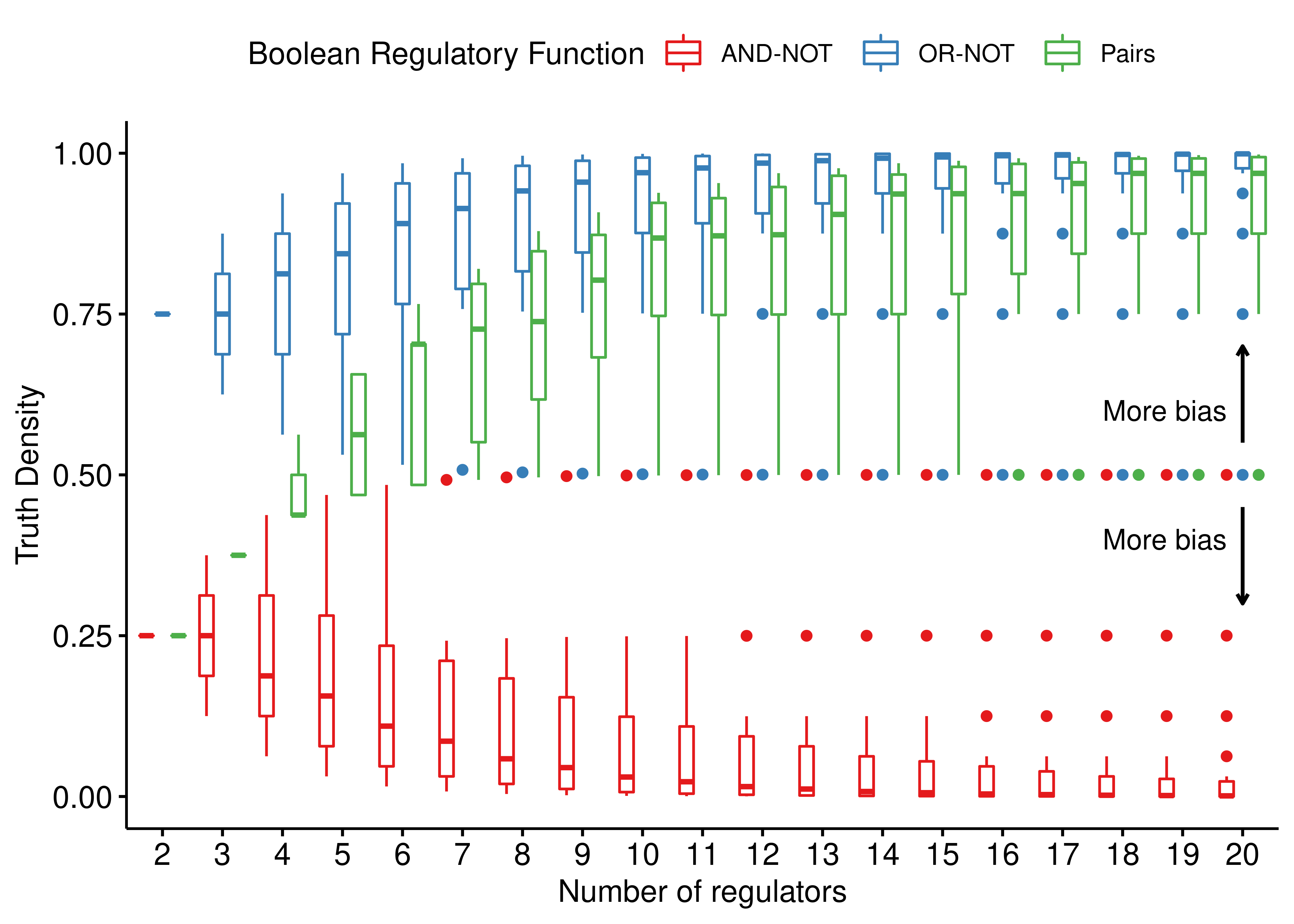

Figure 1: Comparing the truth densities of 3 link operator Boolean regulatory functions: AND-NOT, OR-NOT and Pairs. For each specific number of regulators, every possible configuration of at least one activator and one inhibitor that add up to that number, results in a different truth table output with its corresponding truth density value. All configurations up to 20 regulators are shown.

• The larger the number of regulators, the more biased the link operator functions are towards \(0\), i.e. target inhibition (“AND-NOT”) and \(1\), i.e. target activation (“OR-NOT”, “Pairs”). The “Pairs” function seems to be less biased compared to the “OR-NOT”, but still for large \(n\) (number of regulators) it practically makes the target active.
• For \(n>6\) regulators, the points outside the boxplots (outliers) correspond to the asymptotic behavior of the truth density formulas shown above where there is imbalance between the number of activators and inhibitors (situations close to the extreme ratio scenarios). As such, when \(k \ll m\), \(TD_{AND-NOT} = \frac12\) and when \(m \ll k\), \(TD_{OR-NOT} = \frac12\) - otherwise both functions tend towards more biased outcomes. Interestingly, in both cases of ratio imbalance, the “Pairs” function results in an unbiased truth density output and that is the reason the lower whisker of the corresponding green boxplots touch the unbiased line (with truth density equal to \(0.5\)).

We also check for the relation between truth density and number of activators and inhibitors independently. The following figures demonstrate that the asymptotic behaviour of the truth density of the “AND-NOT” link operator function is largely dependent on the number of inhibitors:

ggscatter(data = stats %>% rename(`#Regulators` = num_reg), x = "num_inh", 
  y = "td_and_not", color = "#Regulators",
  ylab = "Truth Density", xlab = "Number of Inhibitors", 
  title = "AND-NOT TD vs Number of Inhibitors") + 
  theme(plot.title = element_text(hjust = 0.5)) +
  ylim(c(0,1))

ggscatter(data = stats %>% rename(`#Regulators` = num_reg), x = "num_act", 
  y = "td_and_not", color = "#Regulators",
  ylab = "Truth Density", xlab = "Number of Activators", 
  title = "AND-NOT TD vs Number of Activators") + 
  theme(plot.title = element_text(hjust = 0.5)) +
  ylim(c(0,1))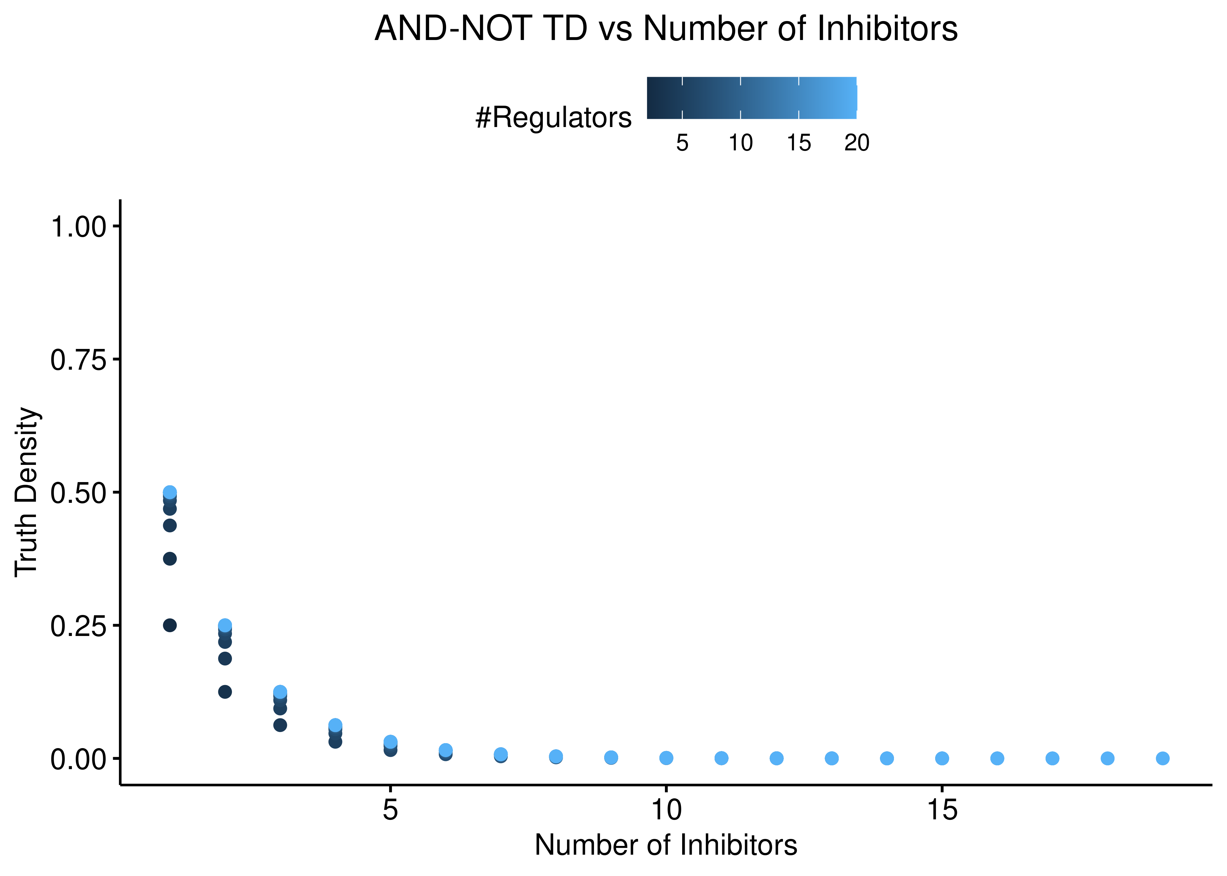

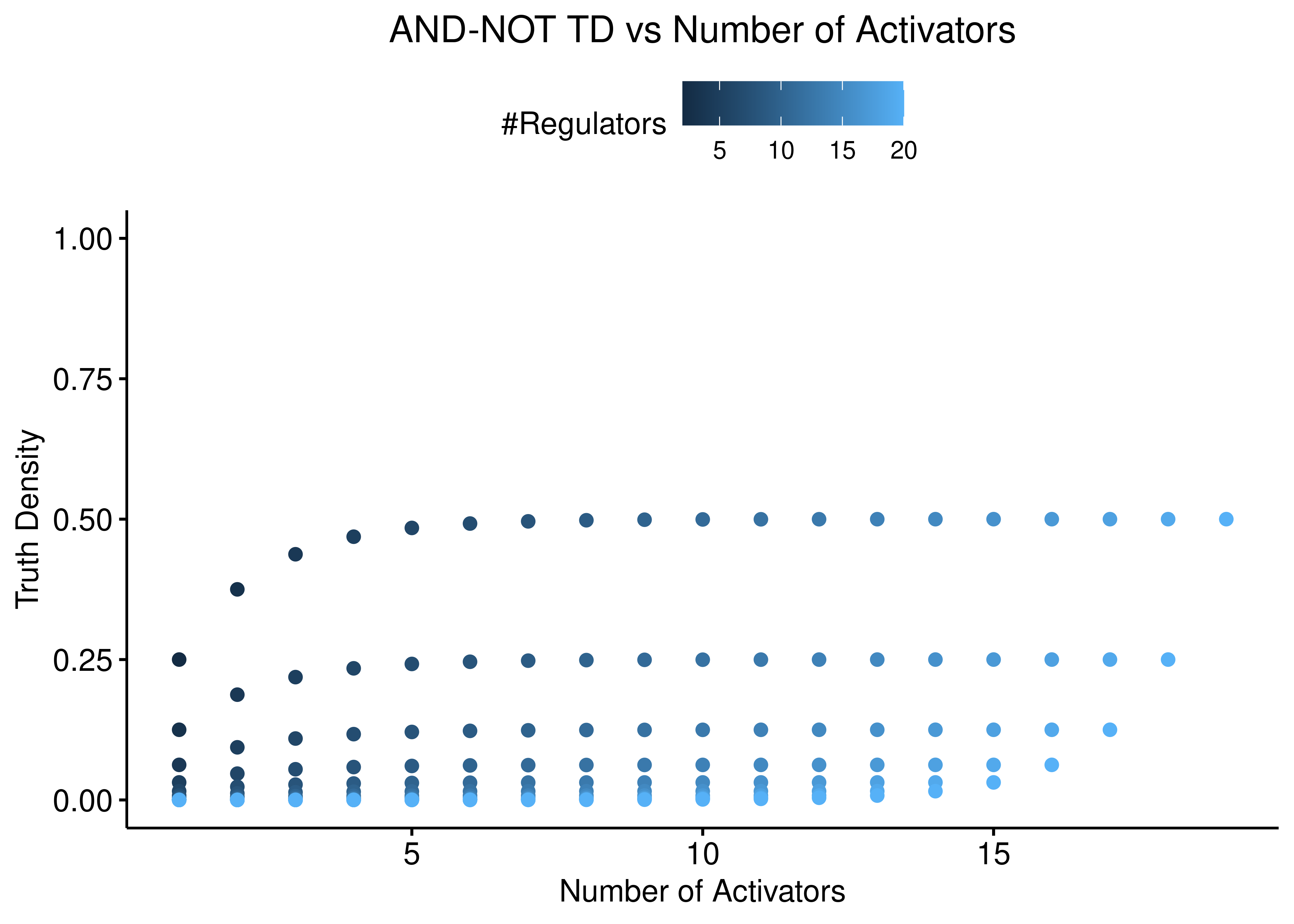
Figure 2: AND-NOT TD vs Number of Activators and Inhibitors

The reverse situation is true for the “OR-NOT” function:

ggscatter(data = stats %>% rename(`#Regulators` = num_reg), 
  x = "num_inh", y = "td_or_not", color = "#Regulators",
  ylab = "Truth Density", xlab = "Number of Inhibitors", 
  title = "OR-NOT TD vs Number of Inhibitors") + 
  theme(plot.title = element_text(hjust = 0.5)) +
  ylim(c(0,1))

ggscatter(data = stats %>% rename(`#Regulators` = num_reg), 
  x = "num_act", y = "td_or_not", color = "#Regulators",
  ylab = "Truth Density", xlab = "Number of Activators", 
  title = "OR-NOT TD vs Number of Activators") + 
  theme(plot.title = element_text(hjust = 0.5)) +
  ylim(c(0,1))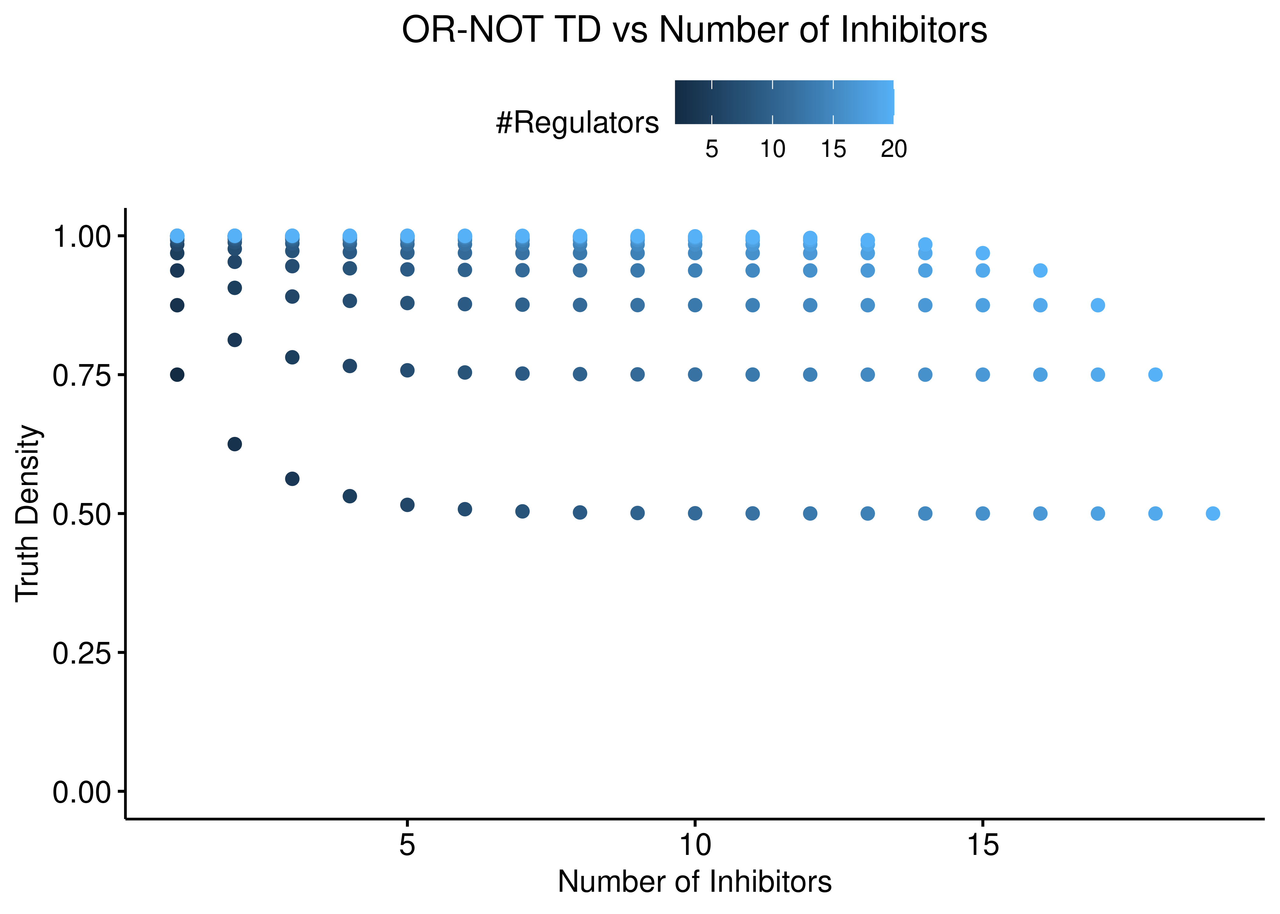

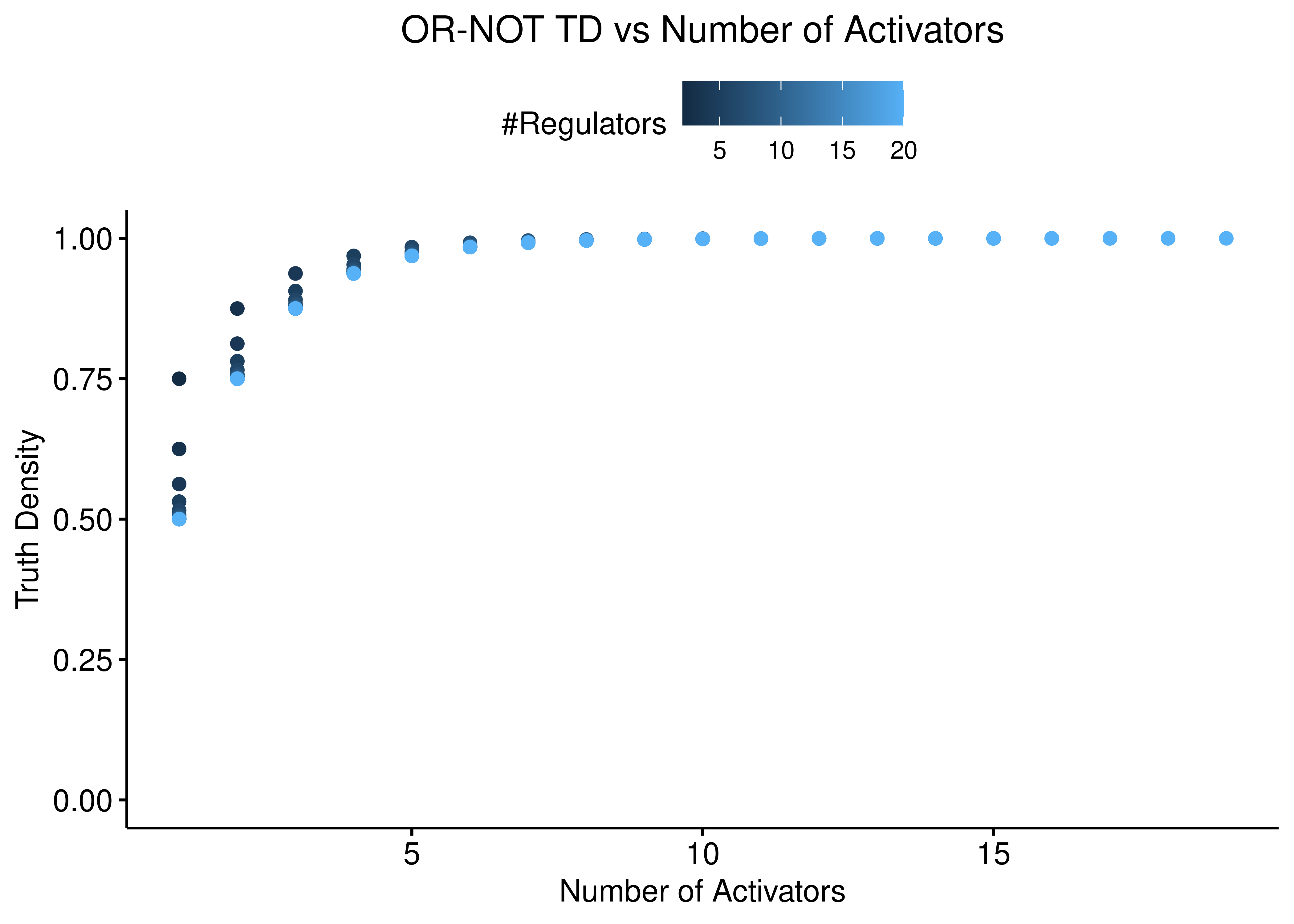
Figure 3: OR-NOT TD vs Number of Activators and Inhibitors

On the other hand, the “Pairs” function shows a more balanced dependency between the number of activators and inhibitors:

ggscatter(data = stats %>% rename(`#Regulators` = num_reg), x = "num_inh", 
  y = "td_pairs", color = "#Regulators",
  ylab = "Truth Density", xlab = "Number of Inhibitors", 
  title = "Pairs TD vs Number of Inhibitors") + 
  theme(plot.title = element_text(hjust = 0.5)) +
  ylim(c(0,1))

ggscatter(data = stats %>% rename(`#Regulators` = num_reg), x = "num_act", 
  y = "td_pairs", color = "#Regulators",
  ylab = "Truth Density", xlab = "Number of Activators", 
  title = "Pairs TD vs Number of Activators") + 
  theme(plot.title = element_text(hjust = 0.5)) +
  ylim(c(0,1))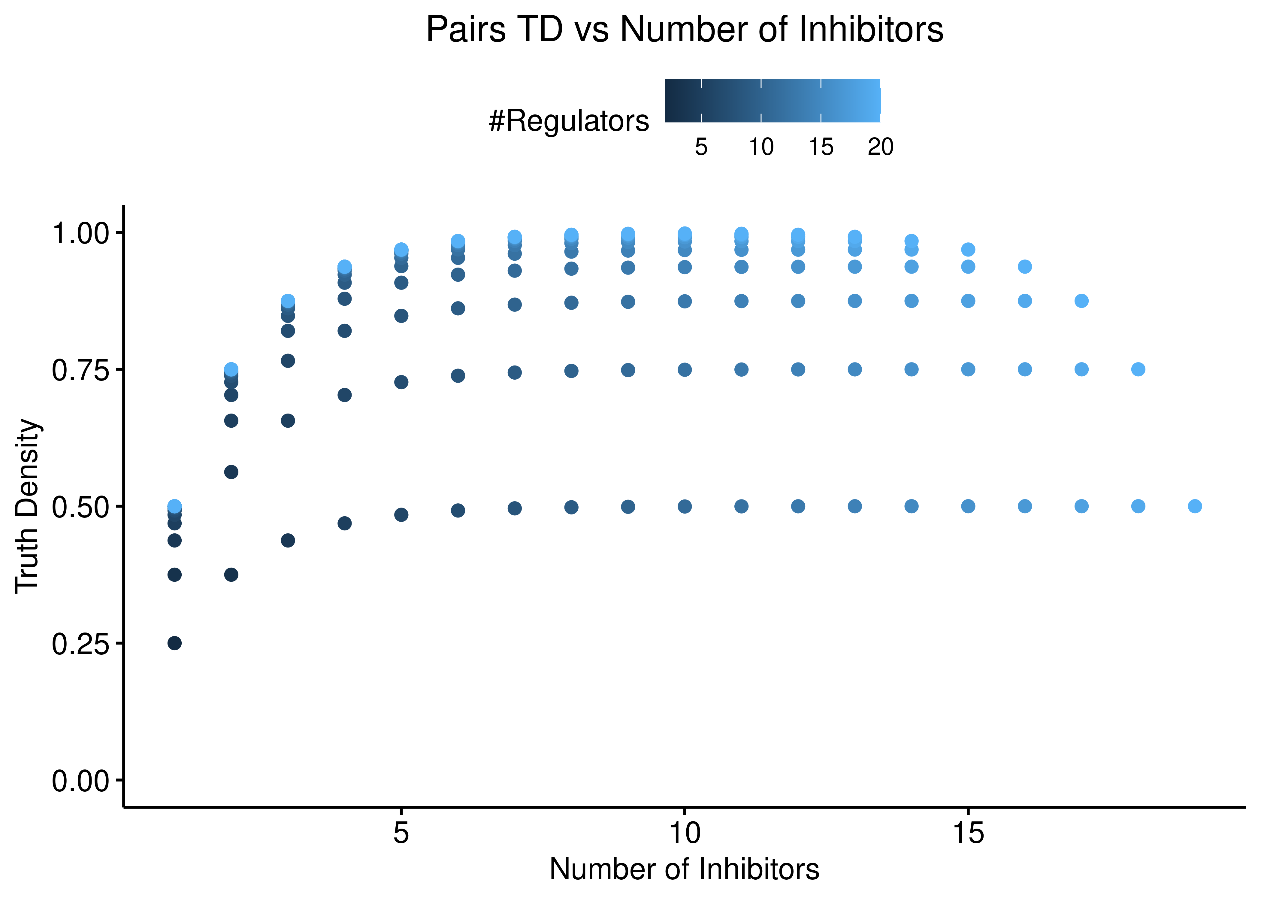

Figure 4: Pairs TD vs Number of Activators and Inhibitors

Threshold functions TD

We check the truth density of the \(f_{Act-win}\) and \(f_{Inh-win}\) Boolean functions:

# tidy up data
stats_functions = tidyr::pivot_longer(data = stats, cols = c(td_act_win, td_inh_win),
  names_to = "fun", values_to = "td") %>%
  select(num_reg, fun, td) %>%
  mutate(fun = replace(x = fun, list = fun == "td_act_win", values = "Activators Win")) %>%
  mutate(fun = replace(x = fun, list = fun == "td_inh_win", values = "Inhibitors Win")) %>%
  rename(`Threshold Function` = fun)

ggboxplot(data = stats_functions, x = "num_reg", y = "td",
  color = "Threshold Function", palette = "lancet",
  #title = latex2exp::TeX("Truth Densities of threshold functions $f_{Act-win}(x,y)$ and $f_{Inh-win}(x,y)$"),
  xlab = "Number of regulators", ylab = "Truth Density") +
  theme(plot.title = element_text(hjust = 0.5)) +
  geom_hline(yintercept = 0.5, linetype = "dashed", color = "black")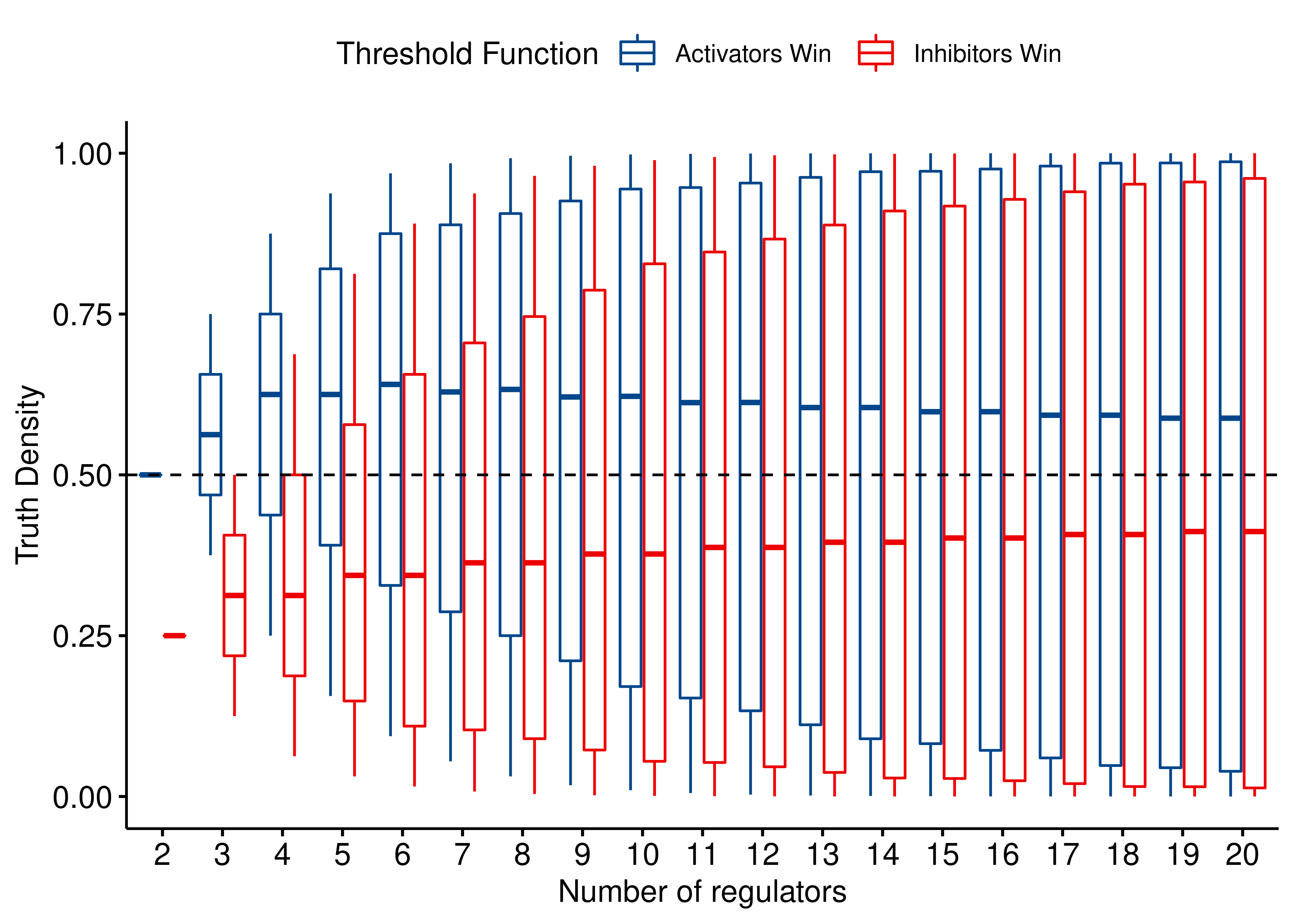

Figure 5: Comparing the truth densities of 2 threshold Boolean regulatory functions: Act-win and Inh-win. For each specific number of regulators, every possible configuration of at least one activator and one inhibitor that add up to that number, results in a different truth table output with its corresponding truth density value. All configurations up to 20 regulators are shown.

• Both Boolean functions show a large variance of truth densities irrespective of the number of regulators, since the values inside the boxplots represent the middle \(50\%\) of the data and span across almost the whole \((0,1)\) range.
• The median truth density values converge to \(1/2\) for both formulas (as was shown in the 1:1 activator-to-inhibitor ratio scenario), which is evidence that these threshold functions behave in a more balanced manner than the other BRFs.
• The median value of truth density for the \(f_{Act-win}\) is always larger than the \(f_{Inh-win}\) (as expected, since the corresponding truth tables have more rows resulting in \(1\), when there are equal number of present activators and inhibitors).

We show the relationship between the two threshold functions TD and the number of inhibitors and activators respectively:

ggscatter(data = stats %>% rename(`#Regulators` = num_reg), x = "num_inh", 
  y = "td_act_win", color = "#Regulators",
  ylab = "Truth Density", xlab = "Number of Inhibitors", 
  title = "Act-win TD vs Number of Inhibitors") + 
  theme(plot.title = element_text(hjust = 0.5)) +
  ylim(c(0,1))

ggscatter(data = stats %>% rename(`#Regulators` = num_reg), x = "num_act", 
  y = "td_act_win", color = "#Regulators",
  ylab = "Truth Density", xlab = "Number of Activators", 
  title = "Act-win TD vs Number of Activators") + 
  theme(plot.title = element_text(hjust = 0.5)) +
  ylim(c(0,1))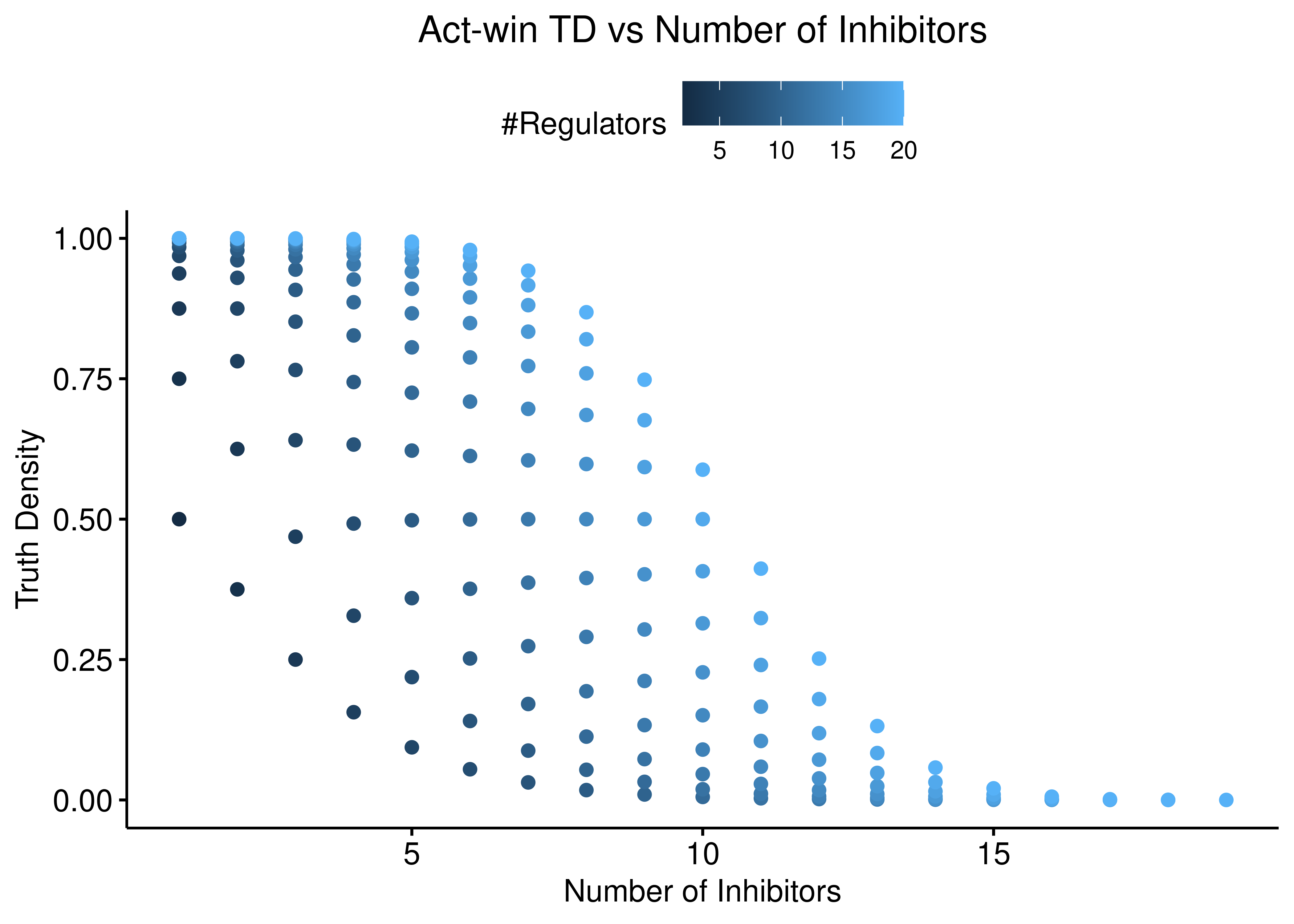

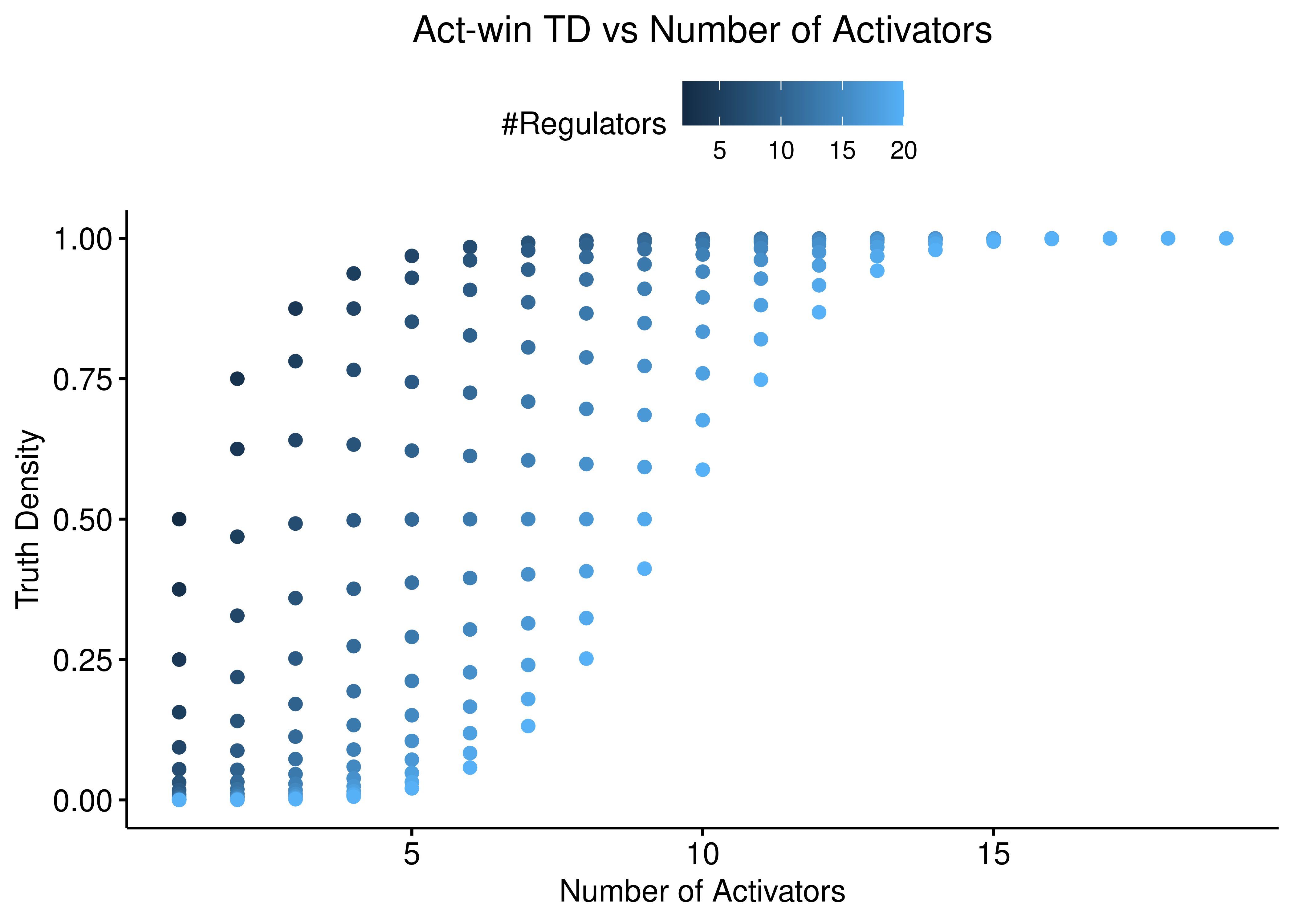
Figure 6: Act-win TD vs Number of Activators and Inhibitors

ggscatter(data = stats %>% rename(`#Regulators` = num_reg), x = "num_inh", 
  y = "td_inh_win", color = "#Regulators",
  ylab = "Truth Density", xlab = "Number of Inhibitors", 
  title = "Inh-win TD vs Number of Inhibitors") + 
  theme(plot.title = element_text(hjust = 0.5)) +
  ylim(c(0,1))

ggscatter(data = stats %>% rename(`#Regulators` = num_reg), x = "num_act", 
  y = "td_inh_win", color = "#Regulators",
  ylab = "Truth Density", xlab = "Number of Activators", 
  title = "Inh-win TD vs Number of Activators") + 
  theme(plot.title = element_text(hjust = 0.5)) +
  ylim(c(0,1))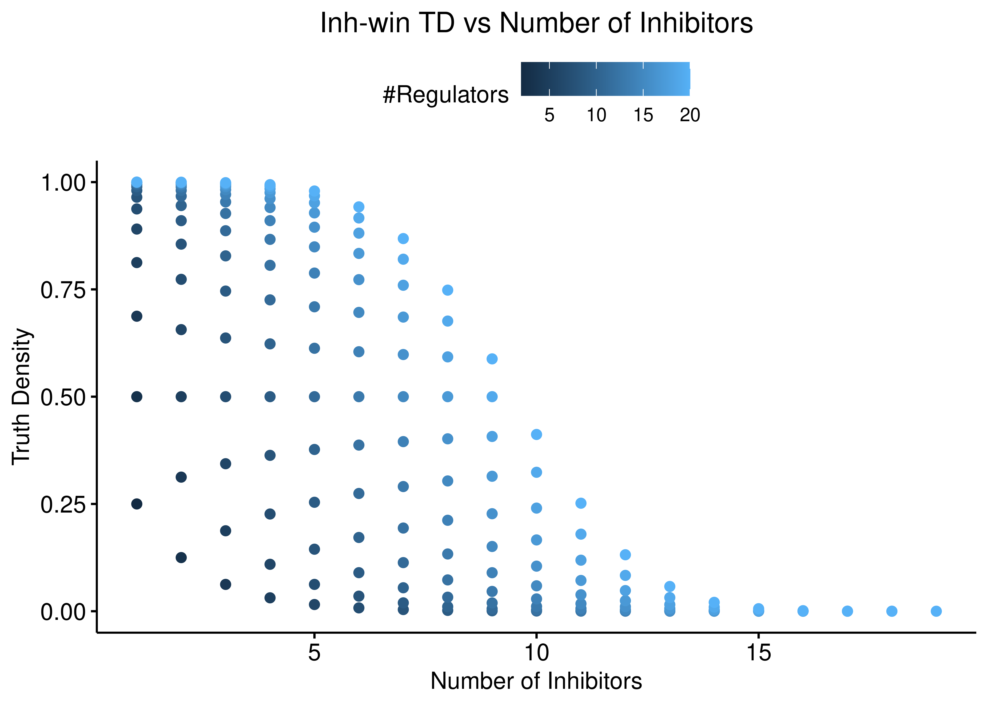

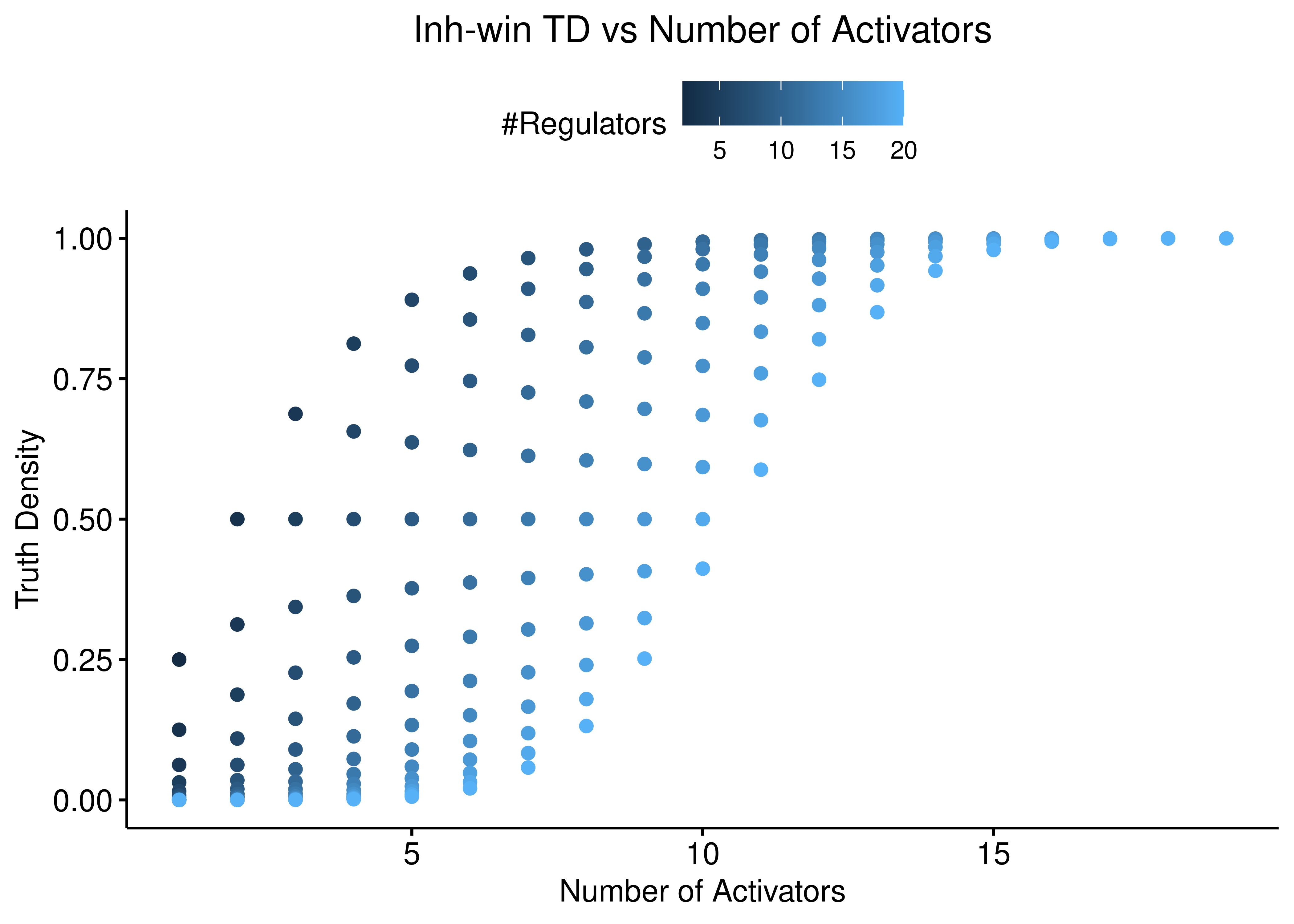
Figure 7: Inh-win TD vs Number of Activators and Inhibitors

Both function behave the same: the more inhibitors (resp. activators), the more biased is the truth density towards \(0\) (resp. \(1\)).

The thickness of the scatterplots is exactly what gives the larger variance/amplitude in the corresponding TD vs #regulators figure, compared to the link operator function results that are more biased.

TD Data Distance

We check how close the truth density values of the different proposed Boolean regulatory functions are to the proportion of activators, e.g. if a function has \(1\) activator and \(5\) inhibitors (resp. \(5\) activators and \(1\) inhibitor) I would expect the Boolean regulatory function’s output to be statistically more inhibited (resp. activated). We find the euclidean distance between the different truth density values and show them in a data table:

x = rbind(`Proportion of Activators` = stats %>% mutate(act_prop = num_act/num_reg) %>% pull(act_prop),
  `AND-NOT TD` = stats %>% pull(td_and_not),
  `OR-NOT TD` = stats %>% pull(td_or_not),
  `Pairs TD` = stats %>% pull(td_pairs),
  `Act-win TD` = stats %>% pull(td_act_win),
  `Inh-win TD` = stats %>% pull(td_inh_win))

d = dist(x, method = "euclidean")

# color `act_prop` column
breaks = quantile(unname(as.matrix(d)[, "Proportion of Activators"]), probs = seq(.05, .95, .05), na.rm = TRUE)
col = round(seq(255, 40, length.out = length(breaks) + 1), 0) %>%
  {paste0("rgb(255,", ., ",", ., ")")} # red

caption.title = "Euclidean Distances between vectors of truth density values (Symmetric)"
DT::datatable(data = d %>% as.matrix(), options = list(dom = "t", scrollX = TRUE),
  caption = htmltools::tags$caption(caption.title, style="color:#dd4814; font-size: 18px")) %>% 
  formatRound(1:6, digits = 3) %>%
  formatStyle(columns = c("Proportion of Activators"), backgroundColor = styleInterval(breaks, col))

plot(hclust(d), main = "Dendogram of Truth Density Distances between various BRFs",
  ylab = "Euclidean Distance", sub = "Boolean Regulatory Functions (BRFs)", xlab = "")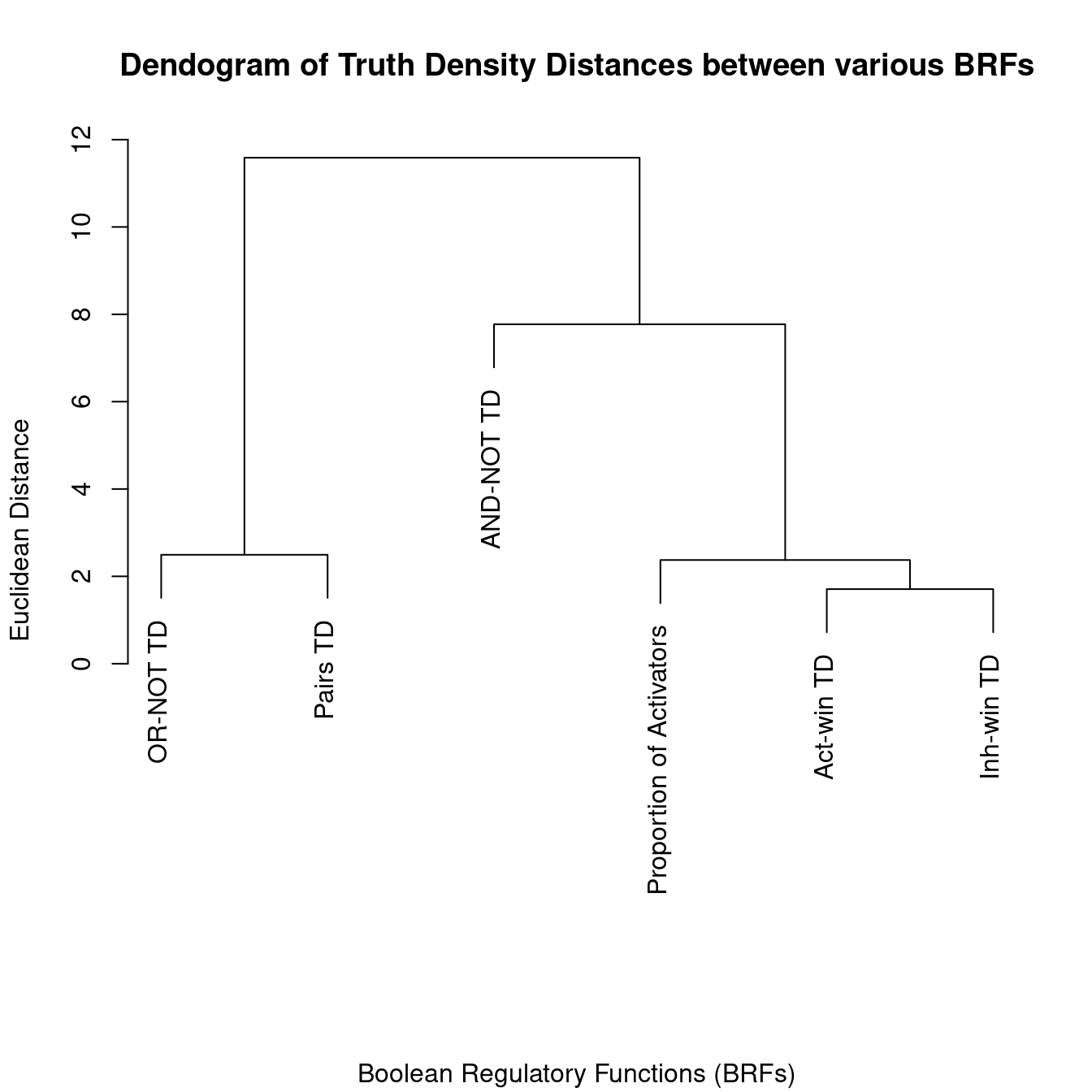

• The threshold functions have truth densities values that are closer to the proportion of activators for a varying number of regulators, compared to the “AND-NOT” and “OR-NOT” formulas. As such they might represent better candidates for Boolean regulatory functions from this (statistical) point of view.
• The TD values of “OR-NOT” and “Pairs” are in general very close (as we’ve also seen in a previous figure)

Complexity vs Truth Density

In (Gherardi and Rotondo 2016), the authors present figures measuring the complexity of Boolean functions based on a formula that counts the number of conjunctions in the minimized DNF form (lets call this \(con_{DNF_{min}}\)) vs the bias (which is their terminology for our truth density!). Since we already have the calculated the TD values for the “AND-NOT”, “OR-NOT” and “Pairs” functions in our test data and their respective (minimum) DNFs (for the “AND-NOT” and “OR-NOT” DNFs see the proofs above and for the “Pairs” DNF, see definition), we can measure the \(con_{DNF_{min}}\) as:

• \(con_{AND-NOT,DNF_{min}} = m\) (number of activators)
• \(con_{OR-NOT,DNF_{min}} = m + 1\) (number of activators + 1)
• \(con_{Pairs,DNF_{min}} = m \times k\) (number of activators x number of inhibitors)

We notice that the “AND-NOT” and “OR-NOT” functions have similar \(con_{DNF_{min}}\) and so we would expect them to have similar complexities, whereas the “Pairs” function should be more complex than both of them.

Dividing the number of conjunctions in the DNF with the number of rows of the corresponding truth table (\(2^n\)), we get the complexity score as defined in (Gherardi and Rotondo 2016). The complexity as it is defined, ranges between \([0,0.5]\), where the highest possible complexity (\(0.5\)) is due to the parity function, which outputs \(1\) for half of the rows in the truth table, i.e. when the number of input \(1\)’s is odd.

Firstly, we calculate the complexity score for each data point:

stats = stats %>% 
  mutate(complex_and_not = num_act/(2^num_reg)) %>%
  mutate(complex_or_not = (num_act + 1)/(2^num_reg)) %>% 
  mutate(complex_pairs = (num_act * num_inh)/(2^num_reg))

Next, we subset the dataset to the Boolean formulas with less than \(10\) regulators and separately to the formulas with more than \(10\) regulators, and group the complexity scores according to the three different functions they belong, namely the “AND-NOT”, “OR-NOT” and “Pairs”:

my_comp = list(c("andnot","ornot"), c("andnot","pairs"), c("ornot","pairs"))

stats %>% 
  filter(num_reg < 10) %>%
  select(starts_with('complex')) %>%
  rename(andnot = complex_and_not, ornot = complex_or_not, pairs = complex_pairs) %>%
  tidyr::pivot_longer(cols = everything(), names_to = 'class', values_to = 'c') %>% 
  ggplot(aes(x = class, y = c, fill = class)) + 
  geom_boxplot(show.legend = FALSE) +
  ggpubr::stat_compare_means(comparisons = my_comp, method = "wilcox.test", label = "p.format") +
  scale_fill_brewer(palette = 'Set1') +
  scale_x_discrete(labels = c('AND-NOT', 'OR-NOT', 'Pairs')) +
  scale_y_continuous(n.breaks = 6) +
  labs(x = 'Function', y = 'Complexity', title = 'Complexity per function class (less than 10 regulators)') +
  theme_classic(base_size = 14) +
  theme(axis.text.x = element_text(size = 12), axis.text.y = element_text(size = 12),
    plot.title = element_text(hjust = 0.5))

stats %>% 
  filter(num_reg > 10) %>%
  select(starts_with('complex')) %>%
  rename(andnot = complex_and_not, ornot = complex_or_not, pairs = complex_pairs) %>%
  tidyr::pivot_longer(cols = everything(), names_to = 'class', values_to = 'c') %>% 
  ggplot(aes(x = class, y = c, fill = class)) + 
  geom_boxplot(show.legend = FALSE) +
  ggpubr::stat_compare_means(comparisons = my_comp, method = "wilcox.test", label = "p.format") +
  scale_fill_brewer(palette = 'Set1') +
  scale_x_discrete(labels = c('AND-NOT', 'OR-NOT', 'Pairs')) +
  scale_y_continuous(n.breaks = 6) +
  labs(x = 'Function', y = 'Complexity', title = 'Complexity per function class (more than 10 regulators)') +
  theme_classic(base_size = 14) +
  theme(axis.text.x = element_text(size = 12), axis.text.y = element_text(size = 12),
    plot.title = element_text(hjust = 0.5))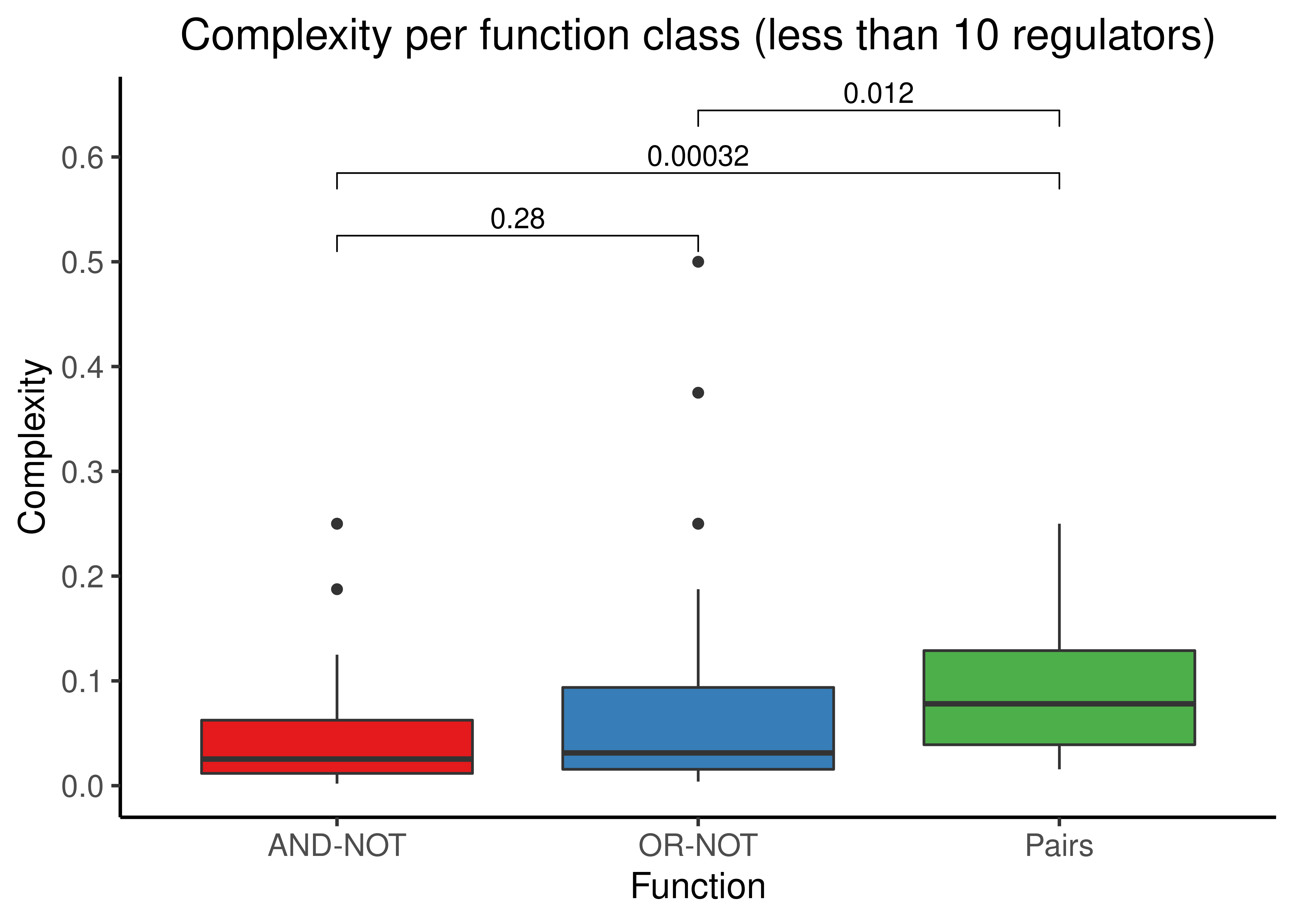

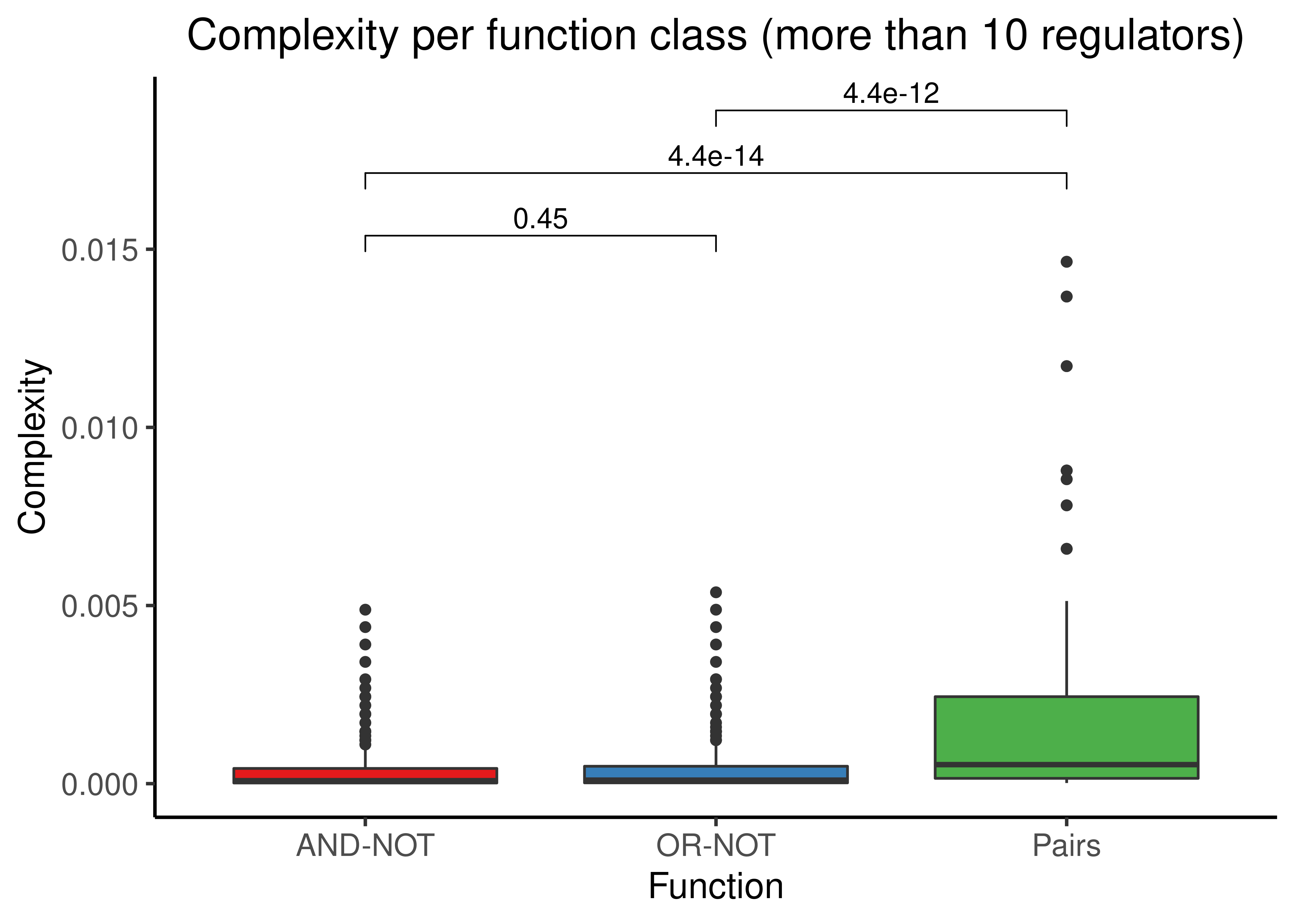
Figure 8: Complexity scores for the AND-NOT, OR-NOT and Pairs Boolean regulatory functions for every Boolean formula with at least one activator and one inhibitor and either less (first figure) or more (second figure) than 10 regulators in total.

• All three functions show low complexities (especially for \(n \gt 10\)), with “Pairs” having the higher median complexity of the three with statistical significance from the other two in both figures.
• The complexities between “AND-NOT” and “OR-NOT” do not differ significantly, as expected from their similar \(con_{DNF_{min}}\) formula.

We next present some Truth Density vs Complexity figures:

stats %>% 
  filter(num_reg < 10) %>%
  select(starts_with('complex'), starts_with('td'), -td_act_win, -td_inh_win) %>% 
  rename(td_andnot = td_and_not, td_ornot = td_or_not, complex_andnot = complex_and_not, complex_ornot = complex_or_not) %>%
  pivot_longer(cols = everything(), names_to = c(".value", "fun"), names_sep = "_") %>% # tricky
  ggplot(aes(x = td, y = complex, color = fun)) +
  geom_point(alpha = 0.6) +
  scale_color_brewer(palette = 'Set1', name = 'Function', 
    labels = c('AND-NOT','OR-NOT','Pairs'), 
    guide = guide_legend(label.theme = element_text(size = 12), 
      override.aes = list(shape = 19, size = 12))) +
  geom_smooth(mapping = aes(x = td, y = complex, fill = fun), method = 'loess', formula = y ~ x, show.legend = FALSE) +
  scale_fill_brewer(palette = 'Set1') + 
  labs(x = 'Truth Density (TD)', y = 'Complexity (C)', title = 'Truth Density vs Complexity (less than 10 regulators)') +
  theme_classic(base_size = 14) +
  theme(axis.text.x = element_text(size = 12), axis.text.y = element_text(size = 12),
    plot.title = element_text(hjust = 0.5))

stats %>% 
  filter(num_reg > 10) %>%
  select(starts_with('complex'), starts_with('td'), -td_act_win, -td_inh_win) %>% 
  rename(td_andnot = td_and_not, td_ornot = td_or_not, complex_andnot = complex_and_not, complex_ornot = complex_or_not) %>%
  pivot_longer(cols = everything(), names_to = c(".value", "fun"), names_sep = "_") %>% # tricky
  ggplot(aes(x = td, y = complex, color = fun)) +
  geom_point(alpha = 0.6) +
  scale_color_brewer(palette = 'Set1', name = 'Function', labels = c('AND-NOT','OR-NOT','Pairs'),
    guide = guide_legend(label.theme = element_text(size = 12), 
      override.aes = list(shape = 19, size = 12))) +
  geom_smooth(mapping = aes(x = td, y = complex, fill = fun), method = 'loess', formula = y ~ x, show.legend = FALSE) +
  scale_fill_brewer(palette = 'Set1') + 
  labs(x = 'Truth Density (TD)', y = 'Complexity (C)', title = 'Truth Density vs Complexity (more than 10 regulators)') +
  theme_classic(base_size = 14) +
  theme(axis.text.x = element_text(size = 12), axis.text.y = element_text(size = 12),
    plot.title = element_text(hjust = 0.5))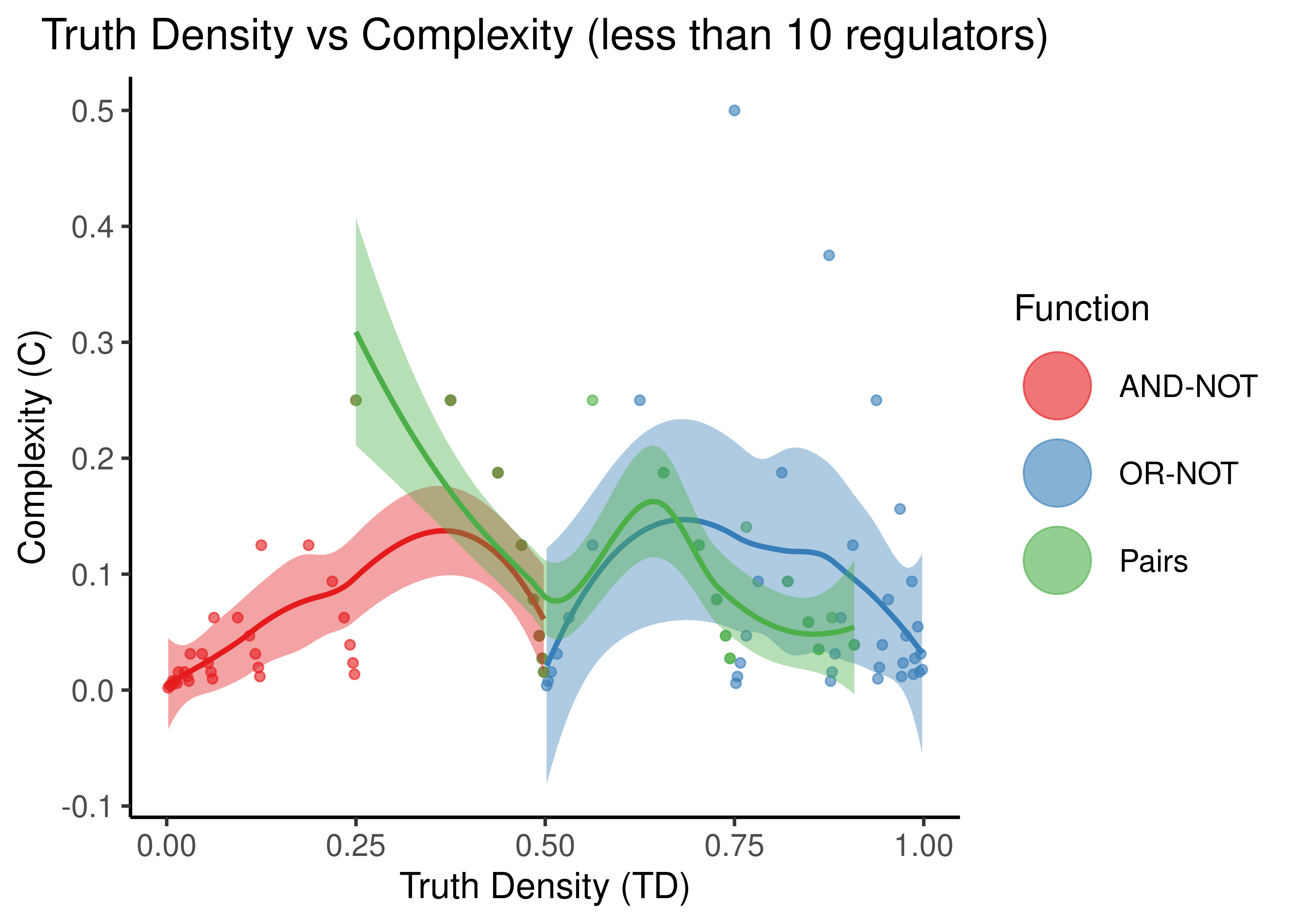

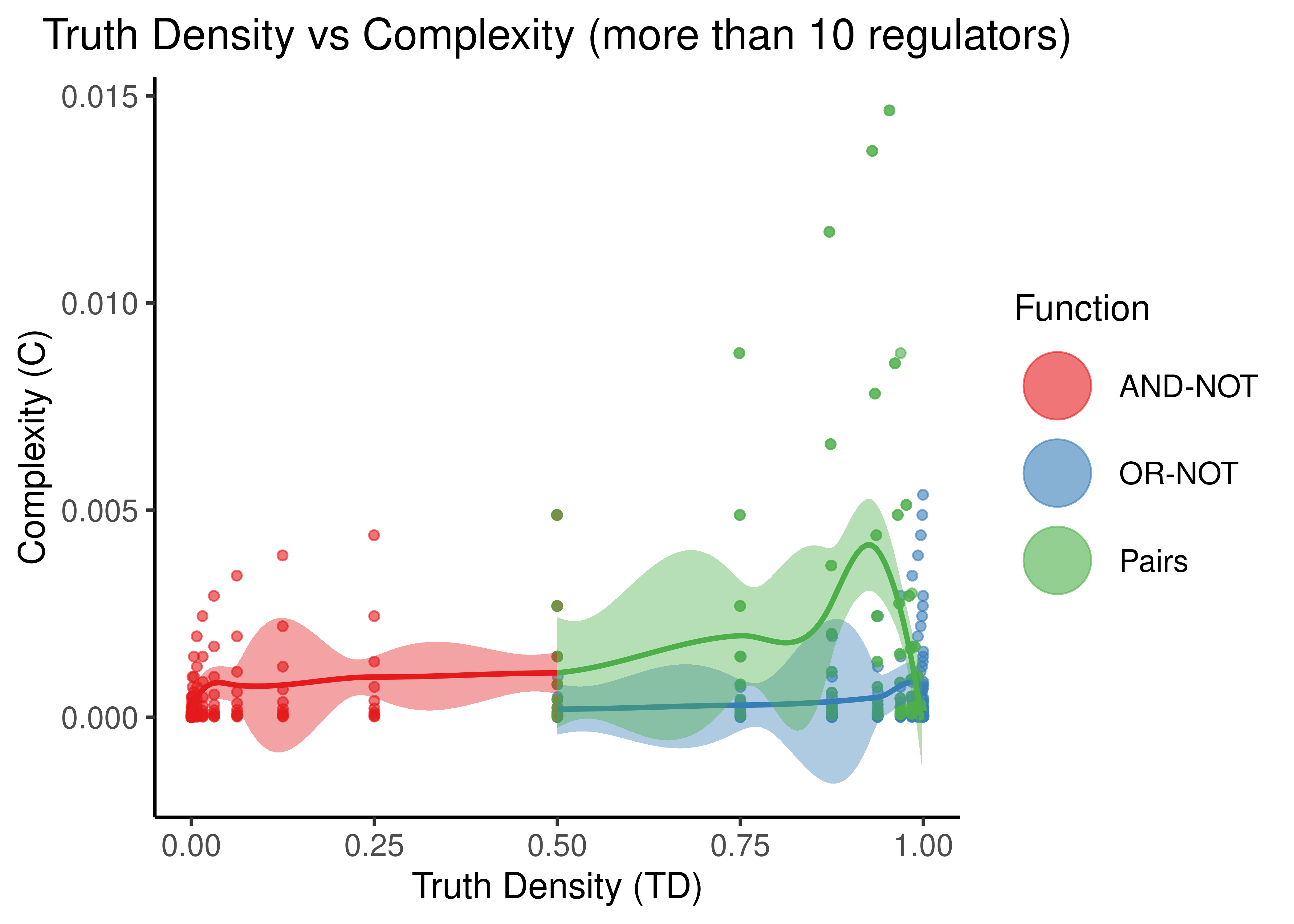
Figure 9: Truth Density vs Complexity for the AND-NOT, OR-NOT and Pairs Boolean regulatory functions. Each point represents a different Boolean formula with at least one activator and one inhibitor. The number of total regulators ranges from 2 to 9 in the first figure and 11 to 20 in the second.

If we put all data together, we have:

stats %>% 
  select(starts_with('complex'), starts_with('td'), -td_act_win, -td_inh_win) %>% 
  rename(td_andnot = td_and_not, td_ornot = td_or_not, complex_andnot = complex_and_not, complex_ornot = complex_or_not) %>%
  pivot_longer(cols = everything(), names_to = c(".value", "fun"), names_sep = "_") %>% # tricky
  ggplot(aes(x = td, y = complex, color = fun)) +
  geom_point(alpha = 0.6) +
  scale_color_brewer(palette = 'Set1', name = 'Function', labels = c('AND-NOT','OR-NOT','Pairs'),
    guide = guide_legend(label.theme = element_text(size = 12), 
      override.aes = list(shape = 19, size = 12))) +
  geom_smooth(mapping = aes(x = td, y = complex, fill = fun), method = 'loess', formula = y ~ x, show.legend = FALSE) +
  scale_fill_brewer(palette = 'Set1') + 
  labs(x = 'Truth Density (TD)', y = 'Complexity (C)', title = 'Truth Density vs Complexity') +
  theme_classic(base_size = 14) +
  theme(axis.text.x = element_text(size = 12), axis.text.y = element_text(size = 12),
    plot.title = element_text(hjust = 0.5))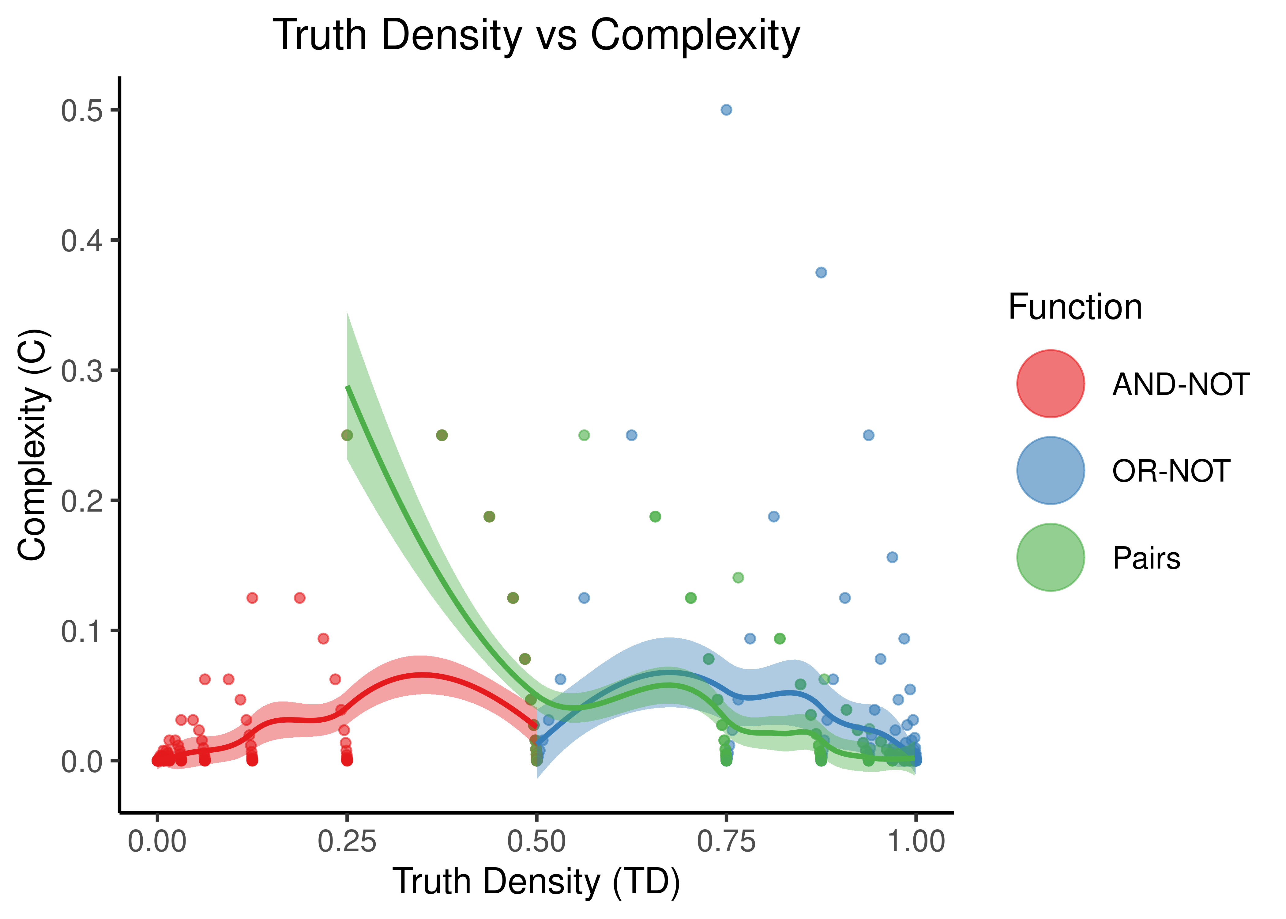

Figure 10: Truth Density vs Complexity for the AND-NOT, OR-NOT and Pairs Boolean regulatory functions. Each point represents a different Boolean formula with at least one activator and one inhibitor. The number of total regulators ranges from 2 to 20 in total.

• “Pairs” covers more TD spectrum than the other two functions, while the “AND-NOT” and “OR-NOT” dichotomize it.
• TD values are very discretized: points tend to cluster at points that denote either the truth density bias (e.g. \(0,1\)) or the cases where there is an unbalance between number of activators and inhibitors (e.g. \(1/2^n\))
• “Pairs” shows higher complexity than the other two functions when the number of regulators is higher (e.g. more than \(10\) regulators) but the difference is not significant since the size of the truth table (\(2^{10}\)) becomes the dominating term in the complexity score. So, in general, as observed in (Gherardi and Rotondo 2016), these Boolean regulatory functions have very low complexity, especially for larger number of regulators.

If we restrict the shown values to a specific number of total regulators, we have the following example figures:

stats %>% 
  filter(num_reg == 5) %>%
  select(starts_with('complex'), starts_with('td'), -td_act_win, -td_inh_win) %>% 
  rename(td_andnot = td_and_not, td_ornot = td_or_not, complex_andnot = complex_and_not, complex_ornot = complex_or_not) %>%
  pivot_longer(cols = everything(), names_to = c(".value", "fun"), names_sep = "_") %>% # tricky
  ggplot(aes(x = td, y = complex, color = fun)) +
  geom_point(alpha = 0.6) +
  scale_color_brewer(palette = 'Set1', name = 'Function', 
    labels = c('AND-NOT','OR-NOT','Pairs'), 
    guide = guide_legend(label.theme = element_text(size = 12), 
      override.aes = list(shape = 19, size = 12))) +
  geom_line(size = 1.2, show.legend = FALSE) +
  labs(x = 'Truth Density (TD)', y = 'Complexity (C)', title = 'Truth Density vs Complexity (5 regulators)') +
  theme_classic(base_size = 14) +
  theme(axis.text.x = element_text(size = 12), axis.text.y = element_text(size = 12),
    plot.title = element_text(hjust = 0.5))

stats %>% 
  filter(num_reg == 8) %>%
  select(starts_with('complex'), starts_with('td'), -td_act_win, -td_inh_win) %>% 
  rename(td_andnot = td_and_not, td_ornot = td_or_not, complex_andnot = complex_and_not, complex_ornot = complex_or_not) %>%
  pivot_longer(cols = everything(), names_to = c(".value", "fun"), names_sep = "_") %>% # tricky
  ggplot(aes(x = td, y = complex, color = fun)) +
  geom_point(alpha = 0.6) +
  scale_color_brewer(palette = 'Set1', name = 'Function', labels = c('AND-NOT','OR-NOT','Pairs'),
    guide = guide_legend(label.theme = element_text(size = 12), 
      override.aes = list(shape = 19, size = 12))) +
  geom_line(size = 1.2, show.legend = FALSE) +
  labs(x = 'Truth Density (TD)', y = 'Complexity (C)', title = 'Truth Density vs Complexity (8 regulators)') +
  theme_classic(base_size = 14) +
  theme(axis.text.x = element_text(size = 12), axis.text.y = element_text(size = 12),
    plot.title = element_text(hjust = 0.5))

stats %>% 
  filter(num_reg == 11) %>%
  select(starts_with('complex'), starts_with('td'), -td_act_win, -td_inh_win) %>% 
  rename(td_andnot = td_and_not, td_ornot = td_or_not, complex_andnot = complex_and_not, complex_ornot = complex_or_not) %>%
  pivot_longer(cols = everything(), names_to = c(".value", "fun"), names_sep = "_") %>% # tricky
  ggplot(aes(x = td, y = complex, color = fun)) +
  geom_point(alpha = 0.6) +
  scale_color_brewer(palette = 'Set1', name = 'Function', labels = c('AND-NOT','OR-NOT','Pairs'),
    guide = guide_legend(label.theme = element_text(size = 12), 
      override.aes = list(shape = 19, size = 12))) +
  geom_line(size = 1.2, show.legend = FALSE) +
  labs(x = 'Truth Density (TD)', y = 'Complexity (C)', title = 'Truth Density vs Complexity (11 regulators)') +
  theme_classic(base_size = 14) +
  theme(axis.text.x = element_text(size = 12), axis.text.y = element_text(size = 12),
    plot.title = element_text(hjust = 0.5))

stats %>% 
  filter(num_reg == 14) %>%
  select(starts_with('complex'), starts_with('td'), -td_act_win, -td_inh_win) %>% 
  rename(td_andnot = td_and_not, td_ornot = td_or_not, complex_andnot = complex_and_not, complex_ornot = complex_or_not) %>%
  pivot_longer(cols = everything(), names_to = c(".value", "fun"), names_sep = "_") %>% # tricky
  ggplot(aes(x = td, y = complex, color = fun)) +
  geom_point(alpha = 0.6) +
  scale_color_brewer(palette = 'Set1', name = 'Function', labels = c('AND-NOT','OR-NOT','Pairs'),
    guide = guide_legend(label.theme = element_text(size = 12), 
      override.aes = list(shape = 19, size = 12))) +
  geom_line(size = 1.2, show.legend = FALSE) +
  labs(x = 'Truth Density (TD)', y = 'Complexity (C)', title = 'Truth Density vs Complexity (14 regulators)') +
  theme_classic(base_size = 14) +
  theme(axis.text.x = element_text(size = 12), axis.text.y = element_text(size = 12),
    plot.title = element_text(hjust = 0.5))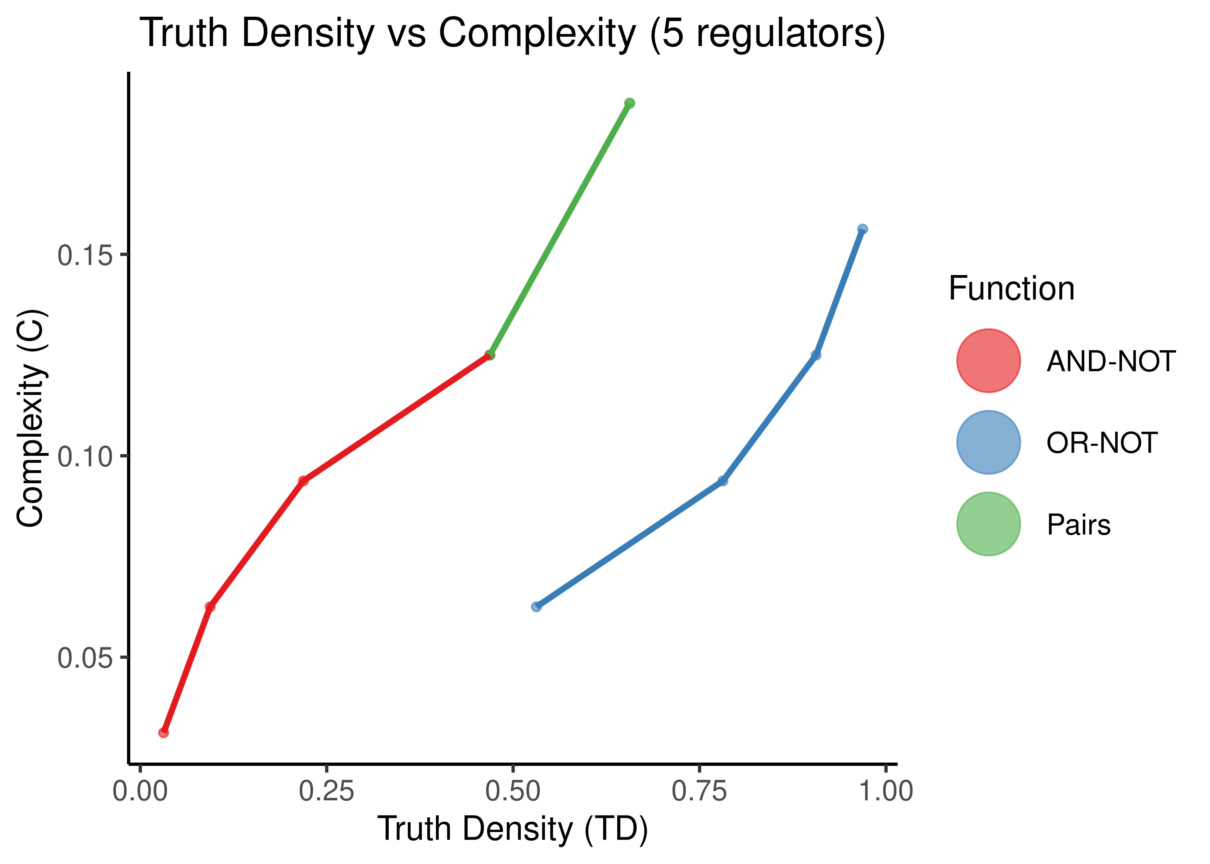

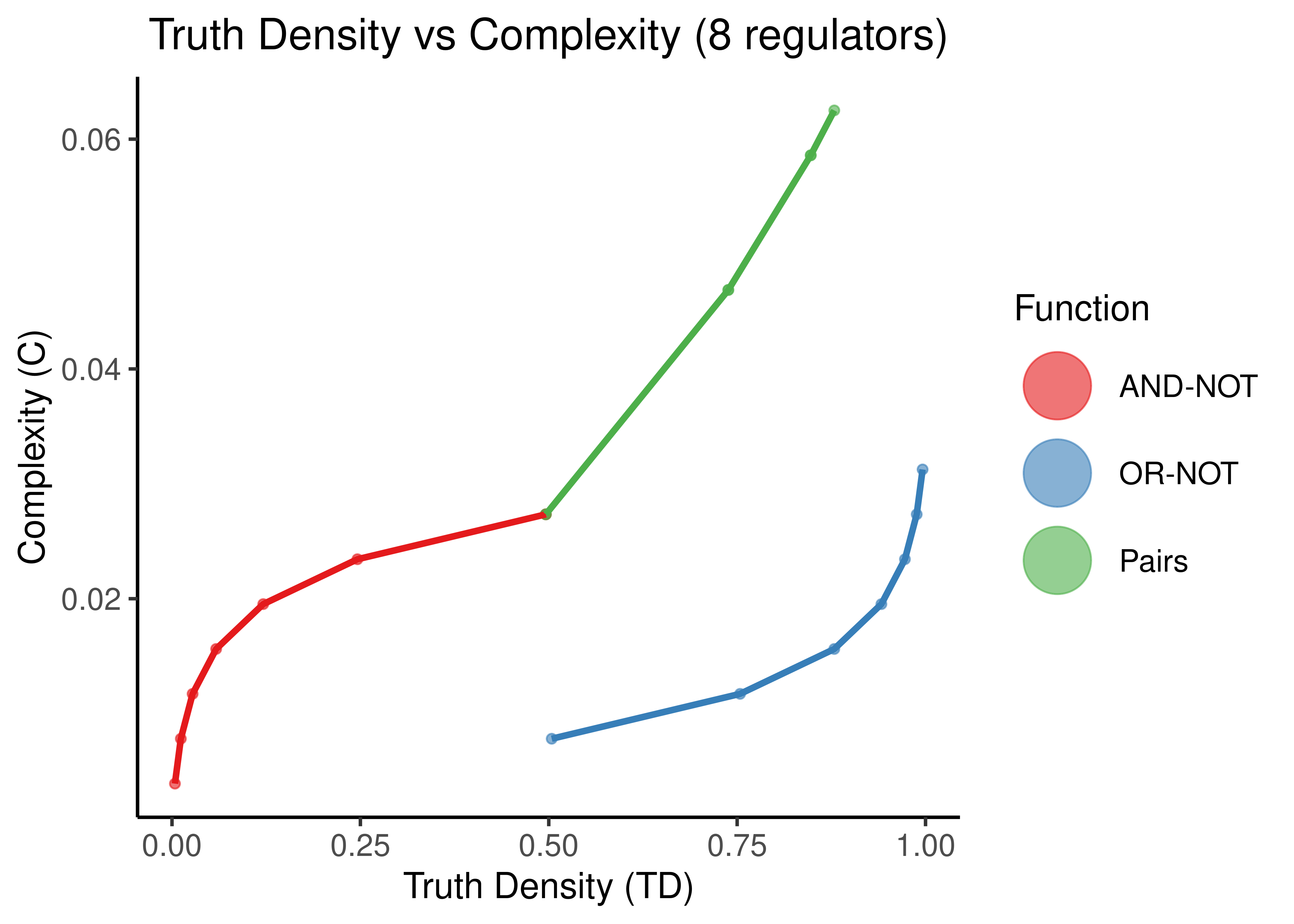
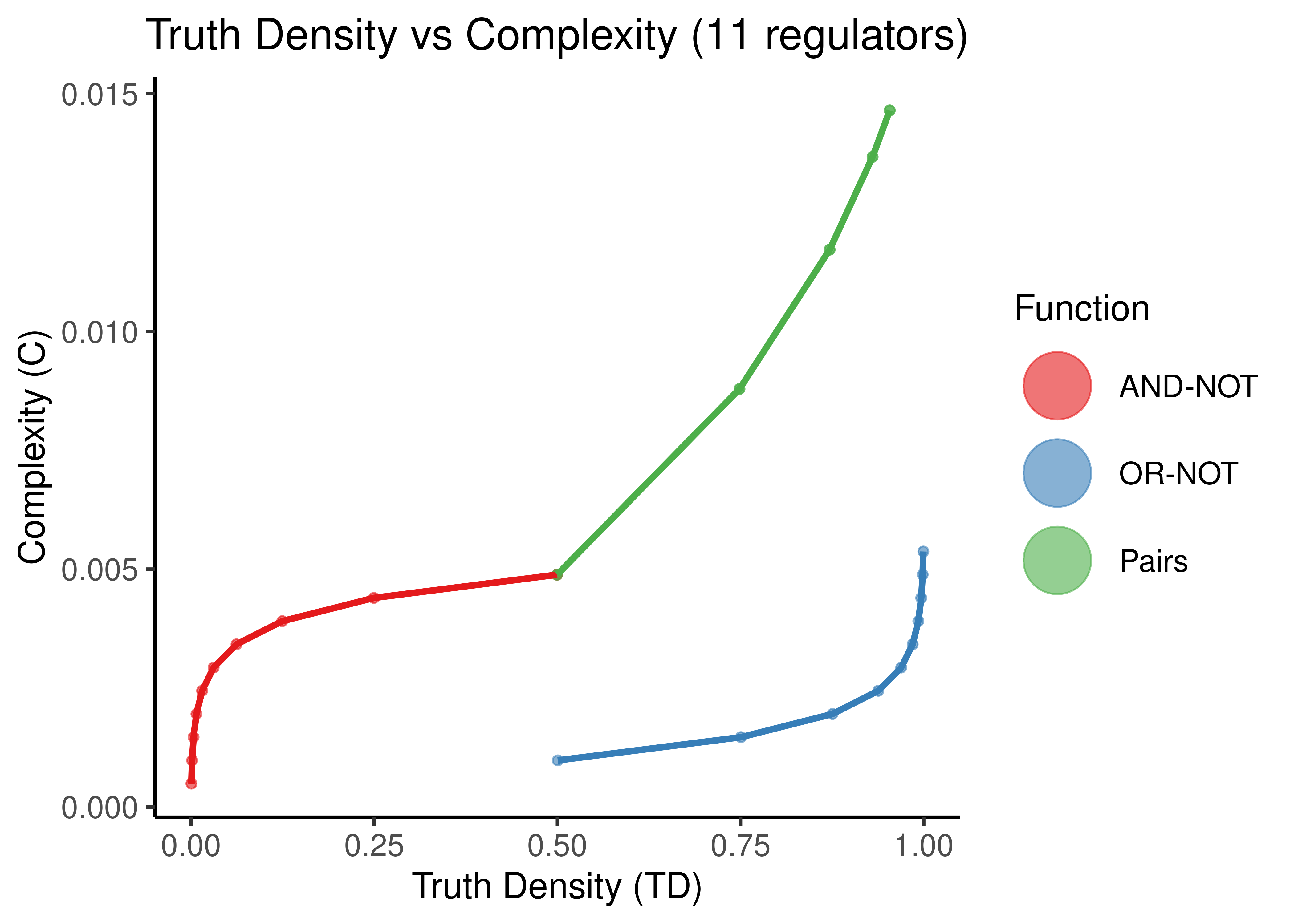
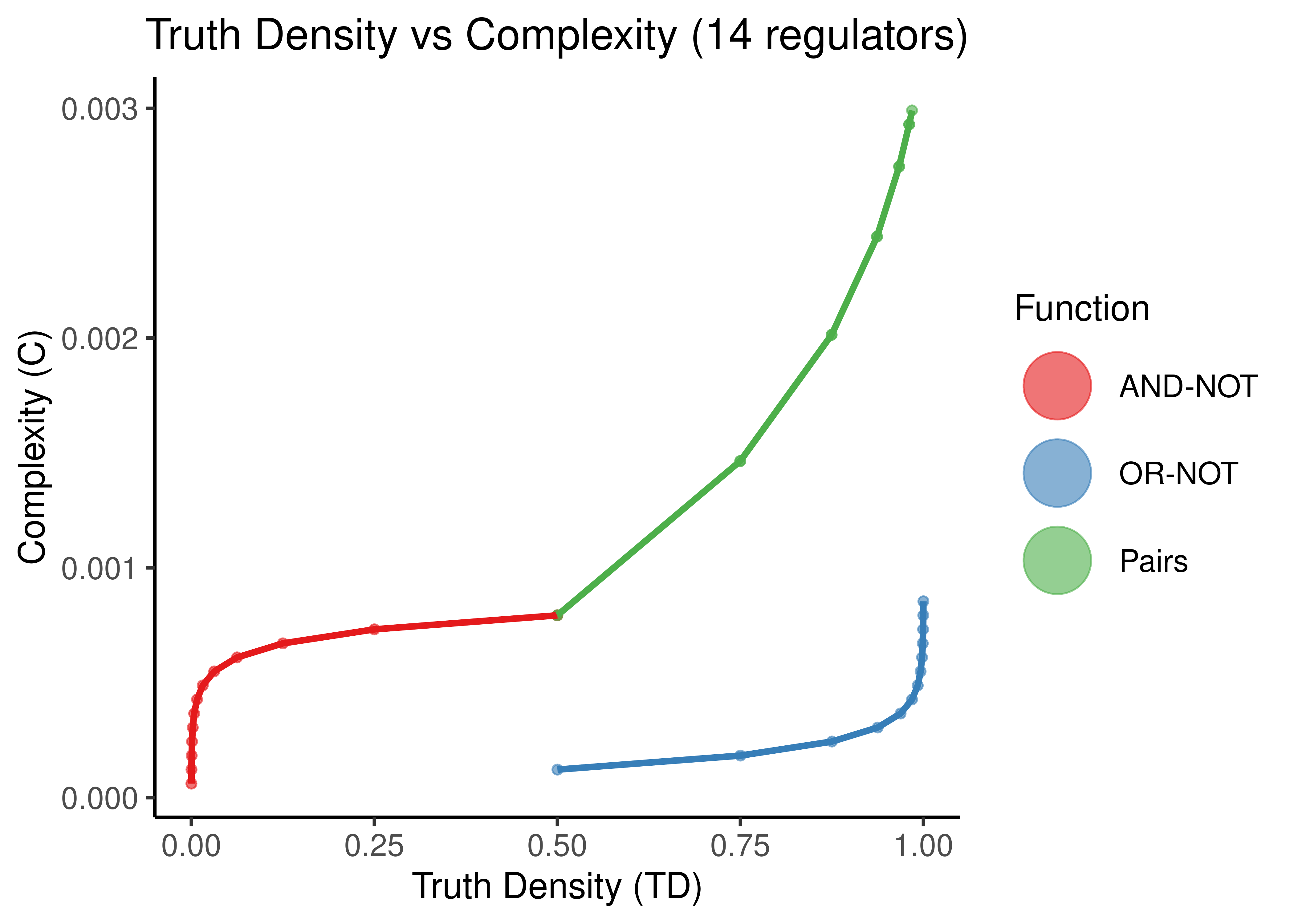
Figure 11: Truth Density vs Complexity for the AND-NOT, OR-NOT and Pairs Boolean regulatory functions. Each point represents a different Boolean formula with at least one activator and one inhibitor. In each figure, formulas with a specific number of total regulators is shown (5,8,11,14).

As observed in (Gherardi and Rotondo 2016) for empirical, experimentally-validated Boolean functions, there seems to be a monotonic relationship between Truth Density and Complexity (when fixing the number of regulators to a particular value).

The more regulators, arbitrarily chosen same-type functions (points here) with different TD values, results in smaller differences of complexity. Also the bias of the “AND-NOT” and “OR-NOT” functions can be visually shown from the large curvature of the red and blue functions for larger number of regulators.