CASCADE 1.0 Data Analysis

Network Properties

In this section we demonstrate the scale-free properties of the CASCADE 1.0 network. We show that both in- and out-degree distributions are asymptotically power-law.

Also, we show that CASCADE 1.0 possesses partial hierarchical modularity.

Use the script get_graph_stats_cascade1.R to generate the degree distribution stats and clustering coefficient scores per node in CASCADE 1.0. We load the results:

graph_stats = readRDS(file = "data/cascade1_graph_stats.rds")

in_stats = graph_stats %>% group_by(in_degree) %>% tally()
# exclude the output nodes with 0 (Antisurvival and Prosurvival)
out_stats = graph_stats %>% group_by(out_degree) %>% tally() %>% slice(-1)

in_stats %>%
  ggplot(aes(x = in_degree, y = n)) +
  geom_bar(stat = "identity", fill = "steelblue", width = 0.7) + 
  geom_smooth(aes(color = "red"), se = FALSE, show.legend = FALSE) + 
  theme_classic() +
  labs(title = "In-Degree Distribution (CASCADE 1.0)", x = "In Degree", y = "Number of Nodes")

out_stats %>%
  ggplot(aes(x = out_degree, y = n)) +
  geom_bar(stat = "identity", fill = "steelblue") + 
  geom_smooth(aes(color = "red"), se = FALSE, span = 0.58, show.legend = FALSE) + 
  theme_classic() +
  labs(title = "Out-Degree Distribution (CASCADE 1.0)", x = "Out Degree", y = "Number of Nodes")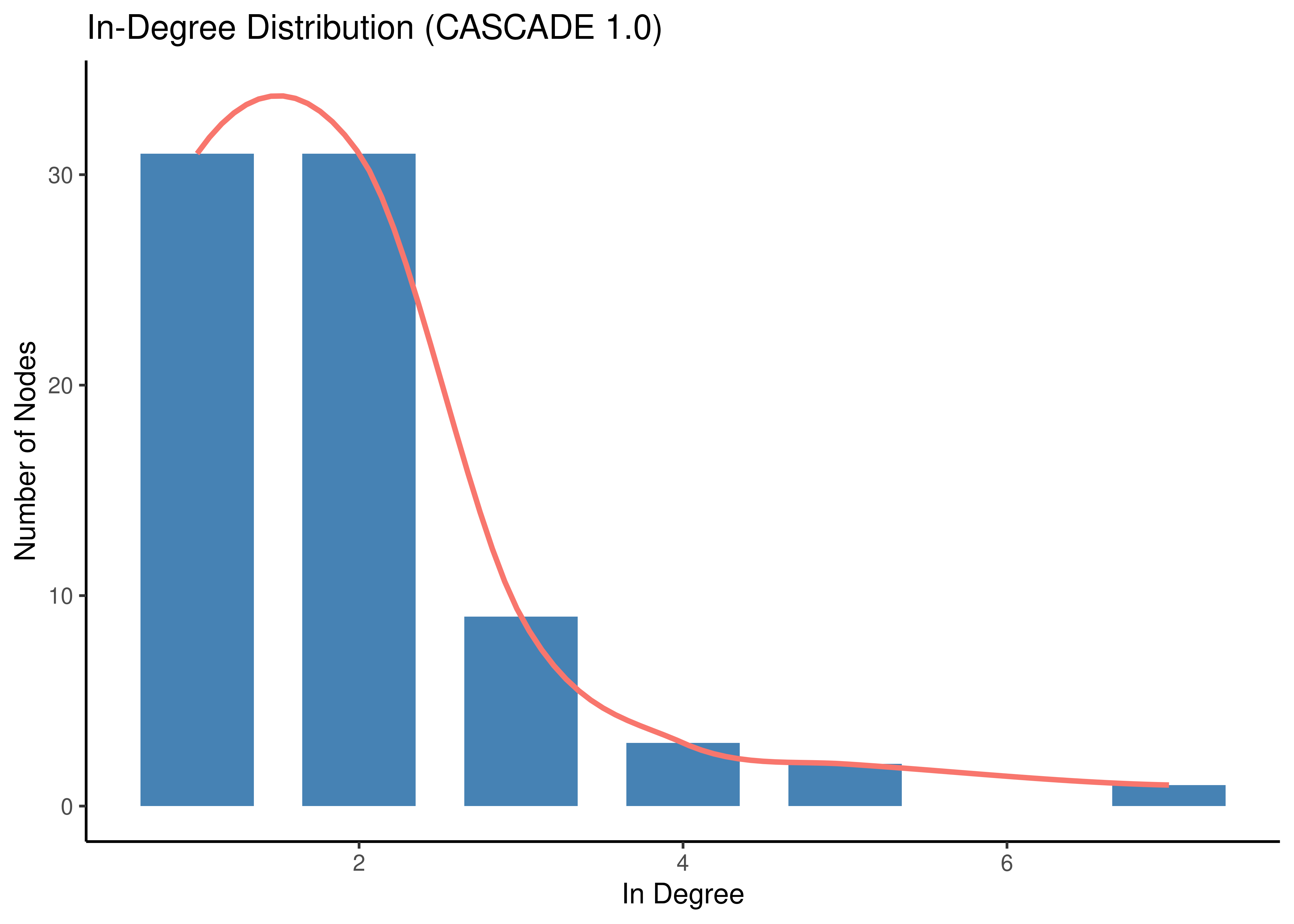

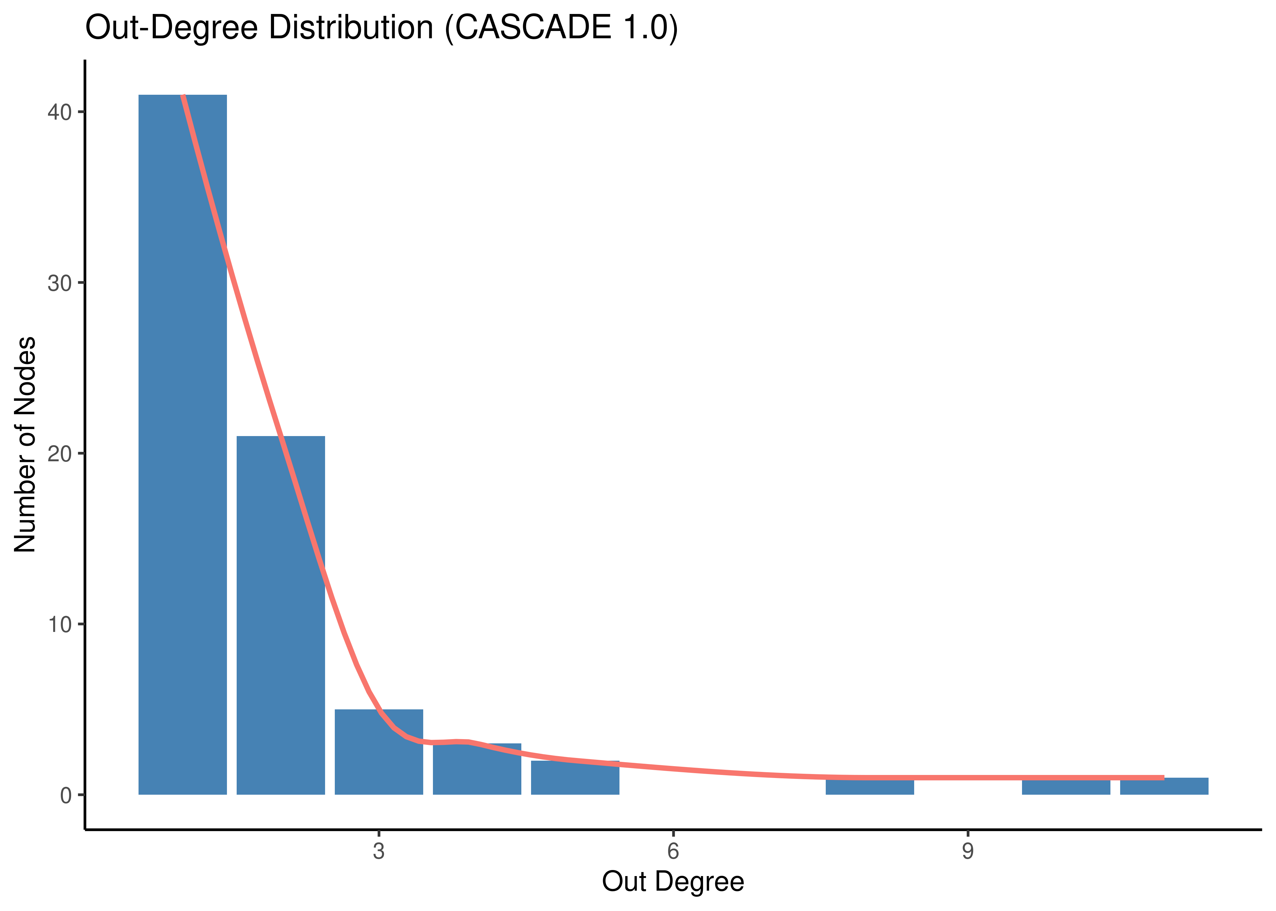
Figure 12: Degree Distribution (CASCADE 1.0)

Degree distributions in a log-log plot are almost straight lines (evidence in favor of the existence of the scale-free property in the CASCADE 1.0 network):

degree_data = dplyr::bind_rows(
  in_stats %>% add_column(degree = 'In') %>% rename(k = in_degree, p_k = n), 
  out_stats %>% add_column(degree = 'Out') %>% rename(k = out_degree, p_k = n)
)

degree_data %>%
  ggplot(aes(x = k, y = p_k, color = degree)) +
  geom_point() + 
  geom_line() +
  labs(x = 'Degree k', y = 'Degree Distribution P(k)') +
  scale_x_log10() +
  scale_y_log10() +
  scale_color_brewer(palette = 'Set1') +
  annotation_logticks(sides = 'bl', outside = FALSE) +
  ggpubr::theme_pubr() +
  theme(legend.position = 'right')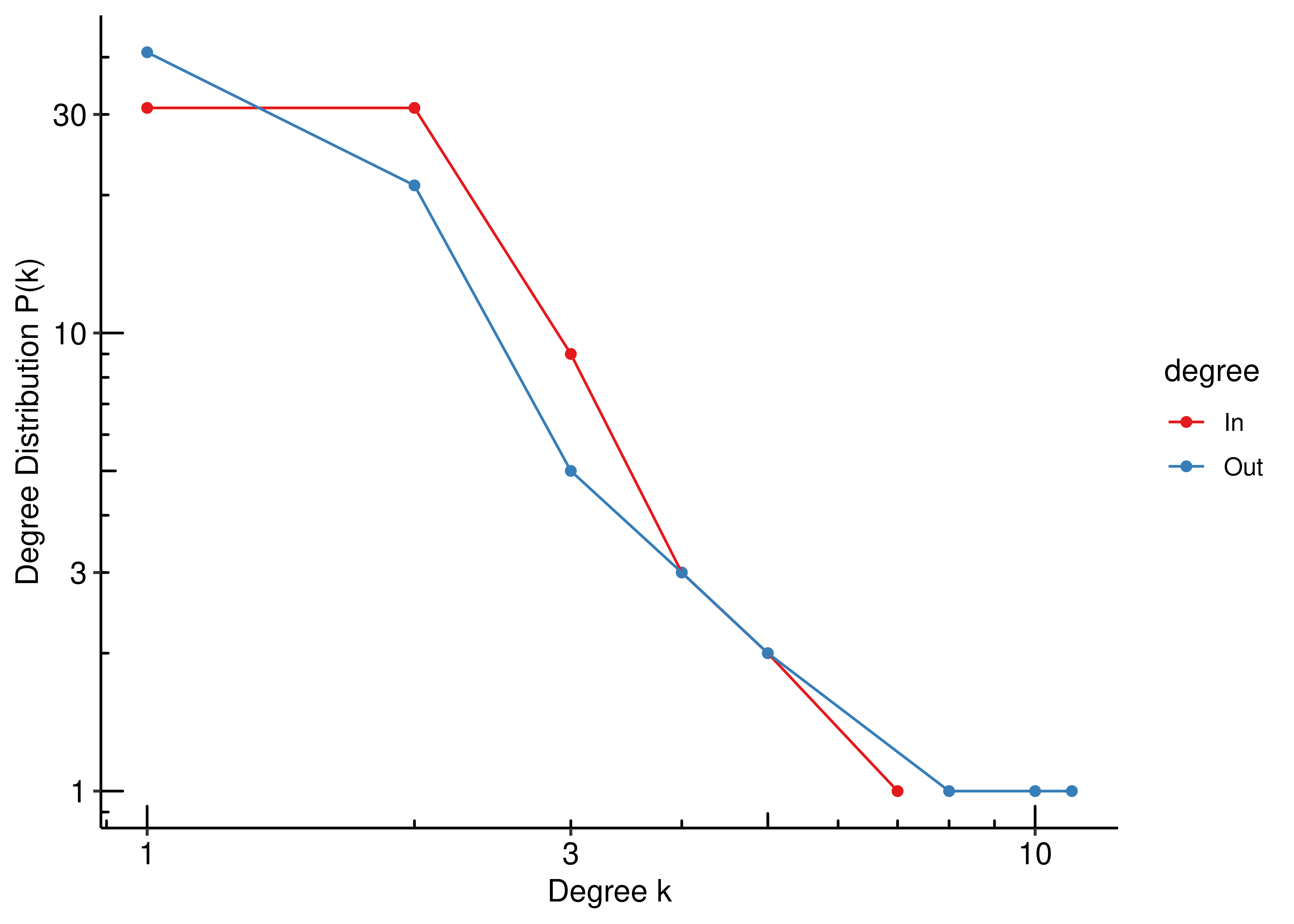

Figure 13: Degree Distribution in a log-log scale (CASCADE 1.0)

Overall, the CASCADE 1.0 network is not hierarchical, since a large fraction of the nodes (\(57/77=74\%\)) has a local clustering coefficient \(C(k)\) equal to \(0\). Most of these nodes have total degrees (sum of in and out degrees) \(2-6\). So, the lower degree nodes are not densely clustered. Also, the network average clustering \(\overline{C}(k)\) is 0.0389783.

In the figure below we show in a log-log plot the clustering coefficient values (excluding the nodes with \(C(k)=0\)). We observe that the \(C(k)\) values decrease linearly with the degree, approximating a straight line with a slope of \(-1\). This suggests hierarchical modularity at least for the higher degree nodes (Ravasz and Barabási 2003).

graph_stats %>% 
  filter(cluster_coef != 0) %>%
  ggplot(aes(x = all_degree, y = cluster_coef)) +
  geom_point() +
  geom_smooth(method = 'lm', formula = y~x, se = FALSE) + 
  scale_x_log10() +
  scale_y_log10() + 
  stat_regline_equation() + 
  labs(x = 'Degree k', y = 'Clustering Coefficient C(k)') +
  ggpubr::theme_pubr()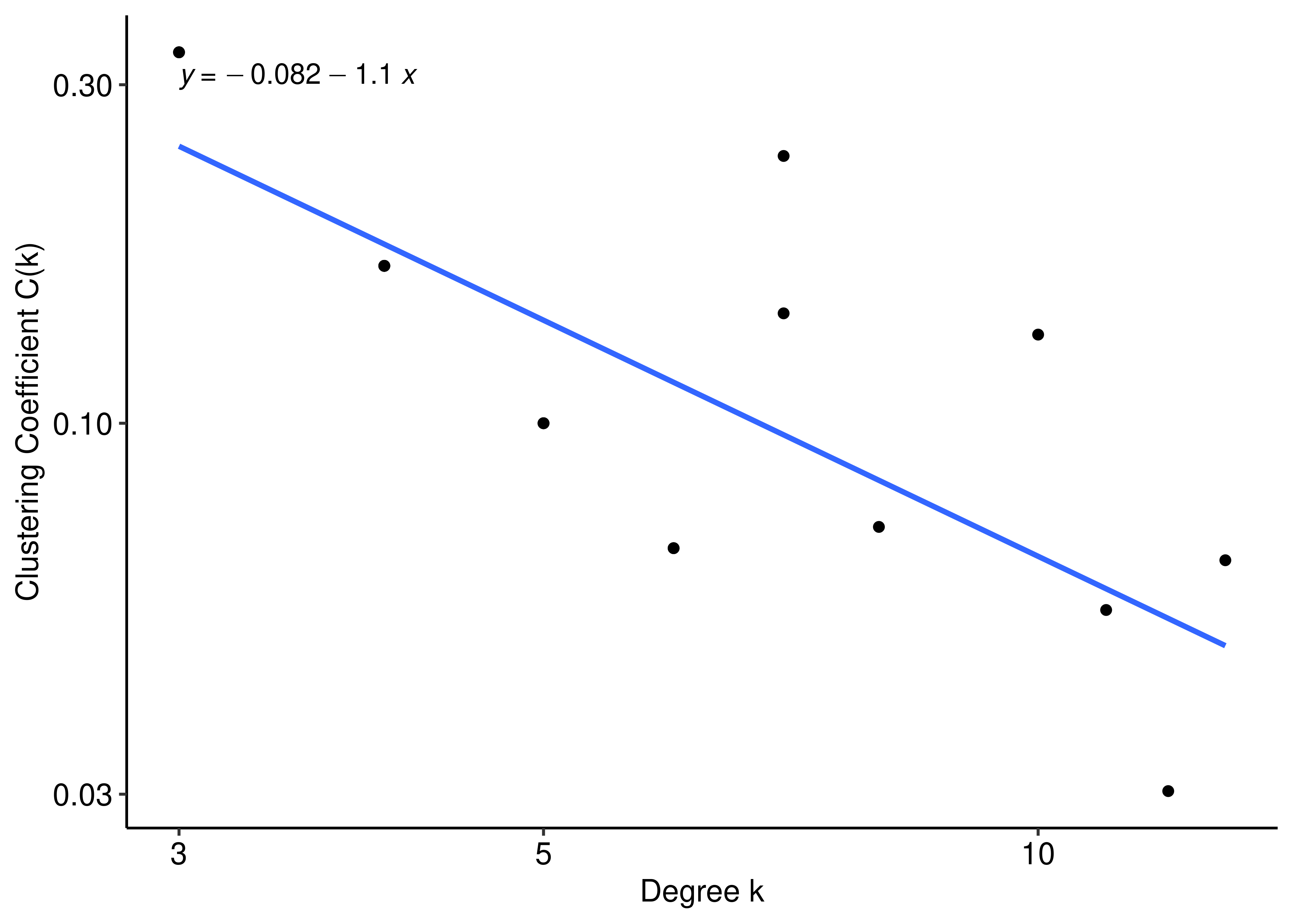

Figure 14: Clustering Coefficient Distribution in a log-log scale (CASCADE 1.0)

Data

Using abmlog we generated all \(2^{23} = 8388608\) possible link operator mutated models for the CASCADE 1.0 topology (\(23\) nodes have at least one regulator from each category, i.e. an activator and an inhibitor). The models are stored in both .gitsbe and .bnet files in the Zenodo dataset (the gitsbe files include also the fixpoint attractors).

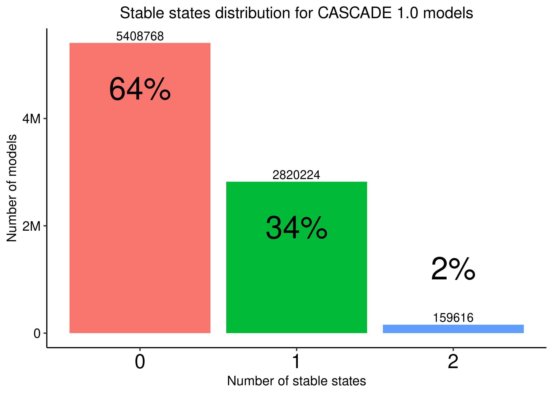
knitr::include_graphics(path = 'img/ss_dist_cascade1.png')

Figure 15: Stable states distribution across all possible link-operator parameterized models generated from the CASCADE 1.0 topology

The dataset includes models with \(0,1\) or \(2\) stable states. We used the get_ss_data.R script to get the 1 stable state data from the models (a total of \(2820224\) models - see figure above, created with the get_ss_dist_stats_cascade1.R) and it’s this data we are going to analyze in the next section.

Parameterization vs Activity

We calculate the node_stats object using the get_node_stats.R script. This object includes the agreement statistics information for each link operator node (i.e. one that is targeted by both activators and inhibitors).

Load the node_stats:

node_stats = readRDS(file = "data/node_stats.rds")

We are interested in two variables of interest:

Parameterization of a link operator node: “AND-NOT” (0) vs “OR-NOT” (1)
Stable State of a node: inhibited (0) vs active (1)

There exist are 4 different possibilities related to 2 cases:

0-0, 1-1 => parameterization and stable state match (e.g. node was parameterized with “AND-NOT” and its state was inhibited or it had “OR-NOT” and its state was active)
1-0, 0-1 => parameterization and stable state differ (e.g. node had “OR-NOT” and its state was inhibited, or “AND-NOT” and its state was active)

The percent Agreement (or total observed proportionate agreement score) is the number of total matches (case 1 above) divided by the total number of data observations/models.

A more robust and sophisticated (compared to the percent agreement) statistic is the Cohen’s kappa coefficient (\(\kappa\)). This statistic is used to measure the extent to which data collectors (raters) assign the same score to the same variable (interrater reliability) and takes into account the possibility of agreement occurring by chance. In our case one rater assigns link operator parameterization (“AND-NOT” or \(0\) vs “OR-NOT” or \(1\)) and the other stable state activity \(0\) vs \(1\)).

In the figures showing Cohen’s \(\kappa\), we draw a horizontal line to indicate the value of \(\kappa=0.6\), above which we have a substantial level of agreement (Landis and Koch 1977; McHugh 2012)

In the next Figure we show the percent agreement for each node:

node_stats %>% mutate(node = forcats::fct_reorder(node, num_reg)) %>% 
  ggplot(aes(x = node, y = obs_prop_agreement, fill = as.factor(num_reg))) +
    geom_bar(stat = "identity") +
    scale_y_continuous(labels=scales::percent) +
    labs(title = "Parameterization and Stable State Agreement", 
      x = "Link operator nodes", 
      y = "Percent Agreement") +
    scale_fill_brewer(guide = guide_legend(reverse = TRUE,
      label.theme = element_text(size = 13),
      title = "Number\nof regulators"), palette = "Set1") +
    geom_hline(yintercept = 0.5, linetype = 'dashed') +
    theme_classic2() + 
    theme(axis.text.x = element_text(angle = 90), 
      plot.title = element_text(hjust = 0.5), legend.position = 'right')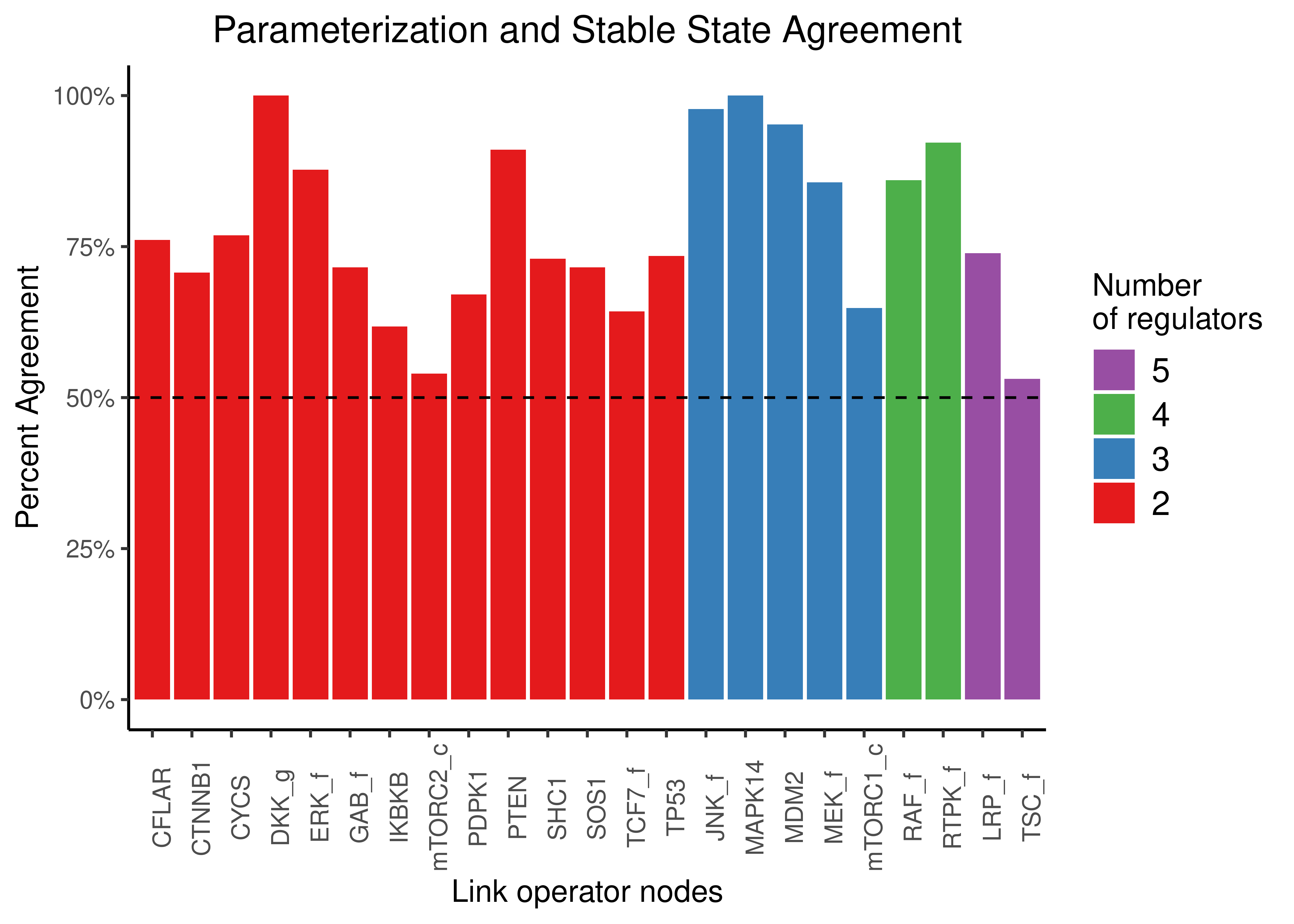

Parameterization and stable state activity agreement for all the CASCADE 1.0 models with one stable state. Only nodes with both activating and inhibiting regulators are shown.

Figure 16: Parameterization and stable state activity agreement for all the CASCADE 1.0 models with one stable state. Only nodes with both activating and inhibiting regulators are shown.

The total barplot area covered (i.e. the total percent agreement score so to speak) is 77.7294779%.

The above score means that the is a higher probability than chance to assign a node the “AND-NOT” (resp. “OR-NOT”) link operator in its respective Boolean equation and that node at the same time having an inhibited (resp. activated) stable state of \(0\) (resp. \(1\)) in any CASCADE 1.0 link operator parameterized model. This suggests that the corresponding Boolean formula used is biased.

In the next figures, we have separated the nodes to groups based on the number of regulators and show both percent agreement and Cohen’s \(\kappa\):

node_stats %>% 
  mutate(num_reg = as.factor(num_reg)) %>%
  ggplot(aes(x = num_reg, y = obs_prop_agreement, fill = num_reg)) + 
    geom_boxplot(show.legend = FALSE) +
    scale_fill_brewer(palette = "Set1") +
    geom_jitter(shape = 19, position = position_jitter(0.2), show.legend = FALSE) +
    scale_y_continuous(labels = scales::percent, limits = c(0,1)) +
    labs(title = "Parameterization and Stable State Agreement", x = "Number of regulators", y = "Percent Agreement") +
    geom_hline(yintercept = 0.5, linetype = 'dashed', color = "red") +
    theme_classic(base_size = 14) +
    theme(axis.text.x = element_text(size = 15), plot.title = element_text(hjust = 0.5))

node_stats %>% 
  mutate(num_reg = as.factor(num_reg)) %>%
  ggplot(aes(x = num_reg, y = cohen_k, fill = num_reg)) + 
    geom_boxplot(show.legend = FALSE) +
    scale_fill_brewer(palette = "Set1") +
    geom_jitter(shape = 19, position = position_jitter(0.2), show.legend = FALSE) +
    ylim(c(0,1)) +
    labs(title = "Parameterization and Stable State Agreement", x = "Number of regulators", y = latex2exp::TeX("Cohen's $\\kappa$")) +
    geom_hline(yintercept = 0.6, linetype = 'dashed', color = "red") +
    geom_text(aes(x = 3.4, y = 0.55), label=latex2exp::TeX("$\\kappa$ = 0.6")) + 
    theme_classic(base_size = 14) +
    theme(axis.text.x = element_text(size = 15), plot.title = element_text(hjust = 0.5))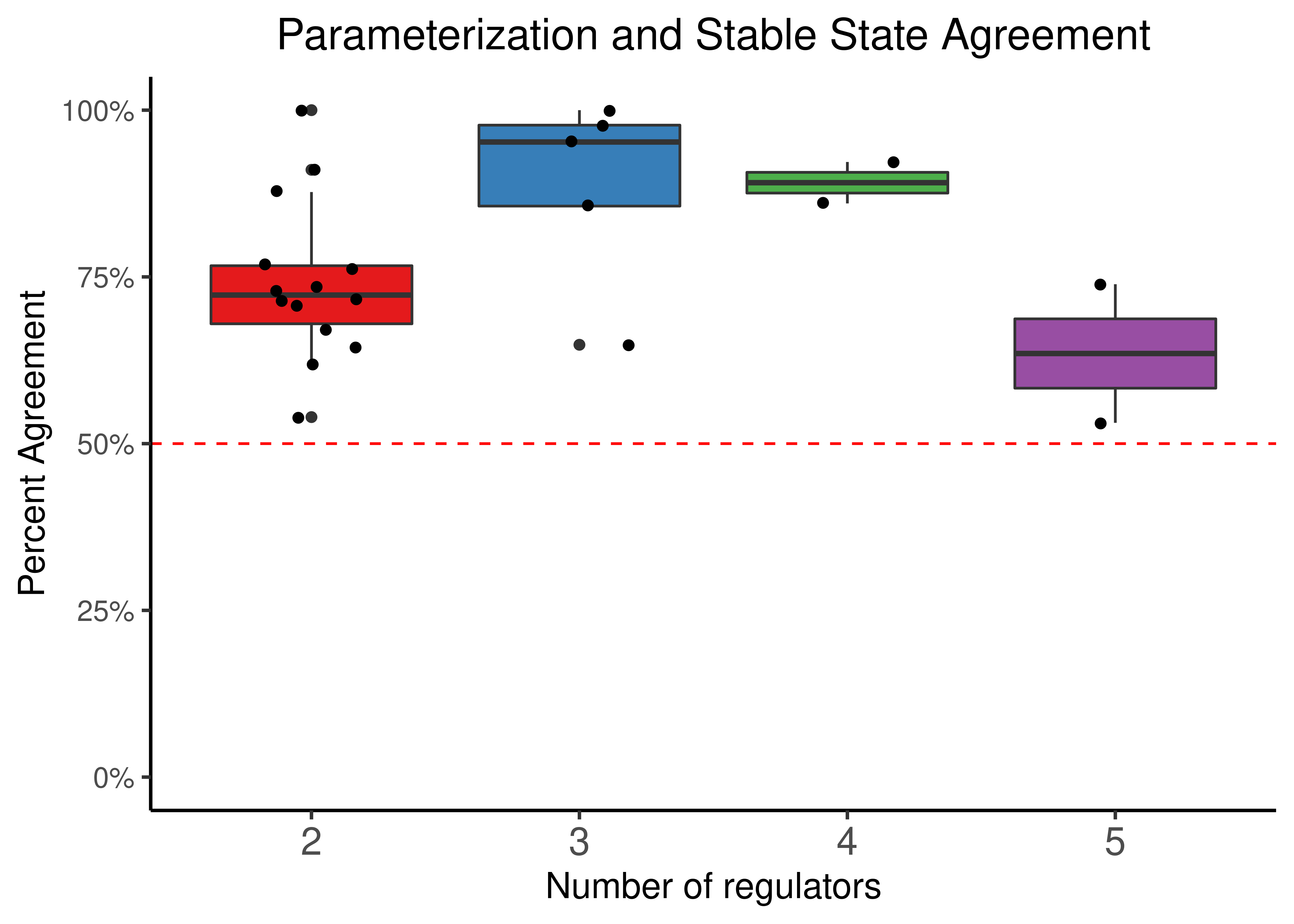

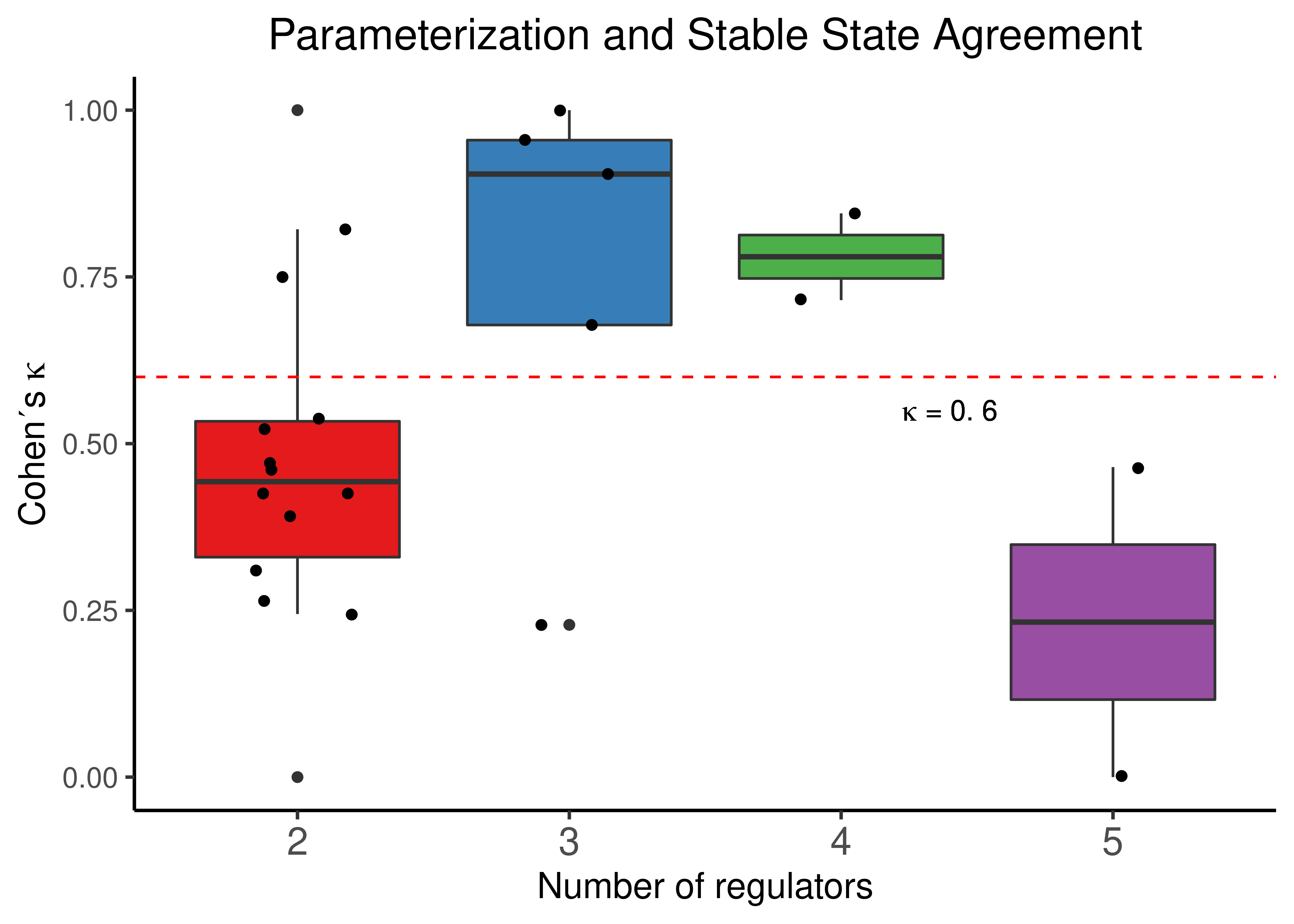
Parameterization and Stable State activity agreement. CASCADE 1.0 link operator nodes are grouped based on their respective number of regulators. Both percent agreement and Cohen's k are presented

Figure 17: Parameterization and Stable State activity agreement. CASCADE 1.0 link operator nodes are grouped based on their respective number of regulators. Both percent agreement and Cohen’s k are presented

We observe that even for a small number of regulators, the median percent agreement score is higher than \(0.5\), though the corresponding Cohen’s \(\kappa\) score seems to be quite variant across the number of regulators.

Since Cohen’s \(\kappa\) is a more strict score to assess agreement between parameterization and stable state activity we conclude that the truth density bias of the standardized regulatory functions might not be quite evident from these data (we need link operator nodes with more regulators).

Next, we calculate per node, the proportion of link operator assignments that retained their expected (i.e. keeping the same digit) stable state activity (e.g. the proportion of models corresponding to the cases 0-0/(0-0 + 0-1) for the “AND-NOT” link operator - and 1-1/(1-1 + 1-0) for “OR-NOT”). We also annotate in the next Figure the nodes experimental activity, which is a results of literature curation (see supplementary material of (Flobak et al. 2015)).

# the AGS steady state
# see https://github.com/druglogics/ags-paper/blob/main/scripts/lo_mutated_models_heatmaps.R#L53
steady_state = readRDS(file = url('https://raw.githubusercontent.com/druglogics/ags-paper/main/data/steady_state.rds'))

# the link operator nodes
# lo_nodes = node_stats %>% pull(node)

# keep only the link operator nodes that belong to the literature-curated steady state
# lo_nodes_in_ss = steady_state[names(steady_state) %in% lo_nodes]

# create stats table
stats_tbl = node_stats %>% 
  mutate(and_not_0ss_prop = and_not_0ss_agreement/(and_not_0ss_agreement + and_not_1ss_disagreement)) %>% 
  mutate(or_not_1ss_prop  = or_not_1ss_agreement/(or_not_1ss_agreement + or_not_0ss_disagreement)) %>%
  select(node, num_reg, and_not_0ss_prop, or_not_1ss_prop, active_prop) %>%
  rename(`AND-NOT` = and_not_0ss_prop, `OR-NOT` = or_not_1ss_prop) %>%
  mutate(node_col = case_when(!node %in% names(steady_state) ~ 'black',
    unname(steady_state[node]) == 0 ~ 'red', TRUE ~ 'green4')) %>%
  mutate(node = forcats::fct_reorder(node, active_prop))

stats_tbl %>% 
  pivot_longer(cols = c(`AND-NOT`, `OR-NOT`)) %>%
  mutate(name = factor(name, levels = c('AND-NOT', 'OR-NOT'))) %>%
  ggplot(aes(x = node, y = value, fill = name)) +
    geom_bar(stat = "identity", position = "dodge") +
    geom_line(aes(x = node, y = active_prop, color = active_prop), group = 1, size = 1.5) + 
    # color = 'Node Activity' trick also works for single line coloring
    # scale_color_manual(name = "", values = c("Node Activity" = "green3"), ) + 
    labs(title = "Parameterization and Stable State Agreement", 
      x = "Link operator nodes", y = "Percent Agreement") +
    scale_fill_brewer(guide = guide_legend(title = "Link Operator", 
      title.theme = element_text(size = 14)), palette = "Set1") + 
    scale_y_continuous(labels = scales::percent, 
      sec.axis = dup_axis(name = 'Average node activity', 
        breaks = c(0,1), labels = c(0,1))) + 
    scale_colour_gradient2(breaks = c(0.2,0.8), labels = c('Inhibited', 'Active'), 
      low = "red", mid = "grey", midpoint = 0.5, high = "green", 
      name = "Activity state", limits = c(0,1), 
      guide = guide_colourbar(title.theme = element_text(size = 14), barheight = 3.5,
        label.theme = element_text(colour = c('red', 'green4')))) +
    theme_classic2() +
    theme(axis.text.x = element_text(angle = 90, 
      color = stats_tbl %>% arrange(active_prop, node) %>% pull(node_col)),
      axis.text.y.right = element_text(face = "bold", color = c('red', 'green4'), size = 16), 
      legend.title = element_text(size = 10),
      plot.title = element_text(hjust = 0.5))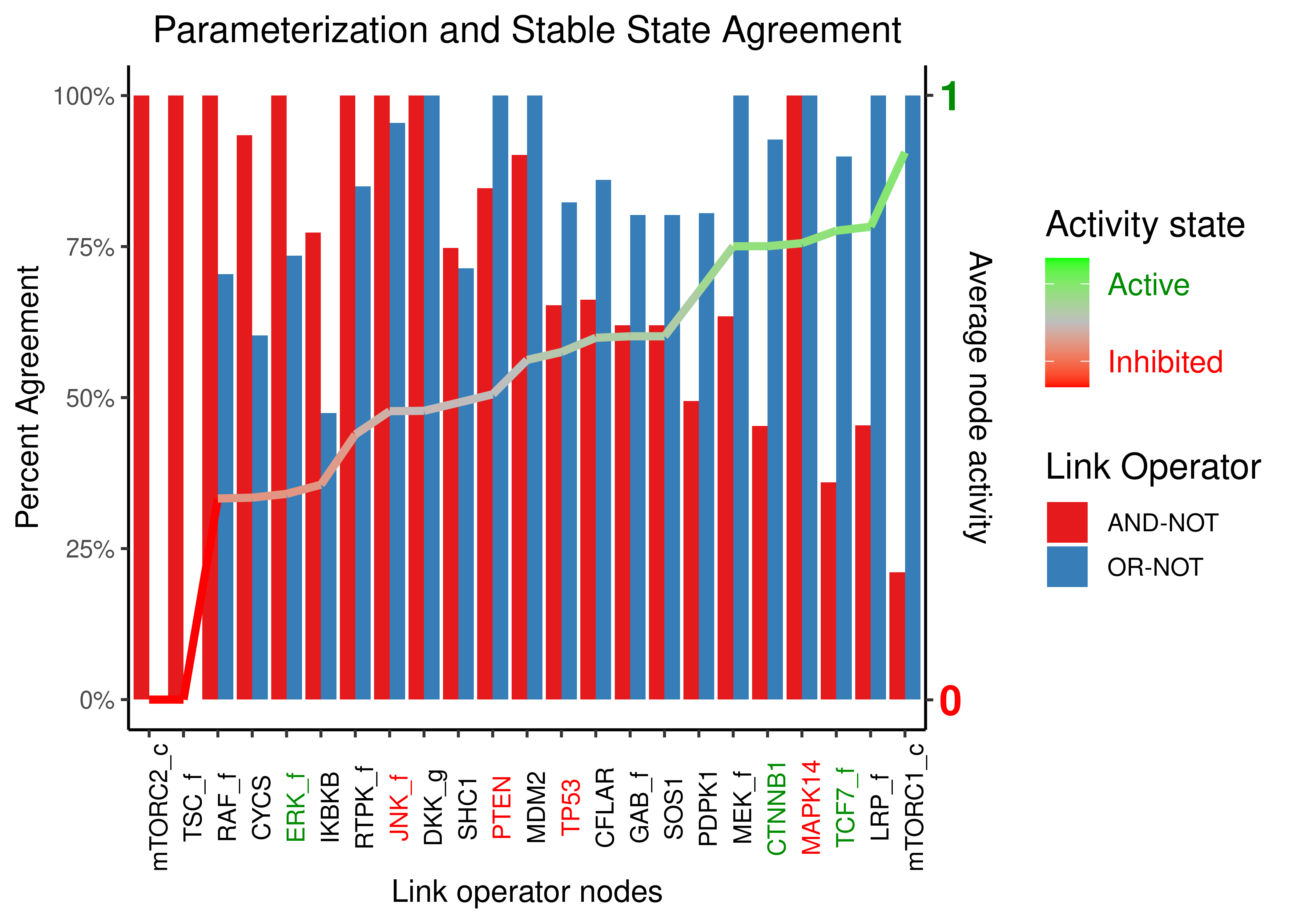

Figure 18: Parameterization and Stable State activity agreement for all the CASCADE 1.0 models with one stable state. Only nodes with both activating and inhibiting regulators are shown. The agreement is splitted per link operator. Nodes are sorted according to the average activity state across all the selected models. We have labeled information about the experimentally observed activity for some of the nodes with green and red, representing active and inhibited states respectively.

Interesting use cases:

For any of the nodes for which we had experimental evidence, a modeler could set the link operator to the appropriate value (in the case of the inhibited nodes JNK_f,PTEN,TP53 and MAPK14 to “AND-NOT” and in the case of the expressed nodes ERK_f, CTNNB1, TCF7_f to “OR-NOT”) and he would have a very high chance that the node would be in same state as denoted by the experimental data in any of the CASCADE 1.0 models with one stable attractor. For example, the data shows that \(90\%\) of the Boolean models whose Boolean equation targeting the node TCF7_f had the “OR-NOT”, also had the node active in their respective stable state. Same for CTNNB1, with a \(92\%\) and ERK_f with the smaller percentage among the active nodes, \(74\%\). All these nodes have 2 regulators (1 activator and 1 inhibitor) and thus \(TD_{AND-NOT,1+1}=0.25\), \(TD_{OR-NOT,1+1}=0.75\) from our truth density analysis. As such, all these nodes behave according to the statistical table results, if not better!
LRP_f has 4 activators and 1 inhibitor and from the previous TD data table we have that: \(TD_{AND-NOT,4+1}=0.469\), \(TD_{OR-NOT,4+1}=0.969\), numbers which correspond really well with the percent agreement scores found across all the CASCADE 1.0 models.
TSC_f and mTORC2_c are always found inhibited and thus the agreement with the “AND-NOT”-inhibited state is perfect and the “OR-NOT”-activated state agreement zero.
TSC_f has 1 activator and 4 inhibitors, which corresponds well to it’s total inhibition profile in all the models (with significantly more inhibitors, there is a higher probability of the target node being inhibited). The TD values are \(TD_{AND-NOT,1+4}=0.03\), \(TD_{OR-NOT,1+4}=0.53\) and so the percent agreement between the “AND-NOT” parameterization and the resulting \(0\) stable state activity is justified, but for the “OR-NOT” cases we would expect around half of them to be in agreement (have a value of \(1\) in the stable state) - which was not the case (all of them had \(0\)). Probably the network dynamical configuration may have something to do with that.

caption.title = "Link Operator Statistics (CASCADE 1.0)"
DT::datatable(data = node_stats %>% select(node, num_reg, num_act, num_inh), 
  caption = htmltools::tags$caption(caption.title, style="color:#dd4814; font-size: 18px"),
  options = list(order = list(list(2, "desc"))))

Node state and percent agreement correlation

We also check for correlation between the average node activity in the CASCADE 1.0 models and the percent agreement per each link operator:

shapiro.test(x = stats_tbl$active_prop)


    Shapiro-Wilk normality test

data:  stats_tbl$active_prop
W = 0.93418, p-value = 0.1347

shapiro.test(x = stats_tbl$`AND-NOT`)


    Shapiro-Wilk normality test

data:  stats_tbl$`AND-NOT`
W = 0.8787, p-value = 0.009442

shapiro.test(x = stats_tbl$`OR-NOT`)


    Shapiro-Wilk normality test

data:  stats_tbl$`OR-NOT`
W = 0.73591, p-value = 4.248e-05

Data seems to be normally distributed since p-values aren’t so much low (for my standards at least :) Use of Pearson’s correlation coefficient is ok in this case.

# individually with ggpubr and kendall coefficent
# ggscatter(data = stats_tbl, x = "active_prop", y = "AND-NOT",
#   xlab = "Average node activity",
#   ylab = "AND-NOT percent agreement",
#   title = "", add = "reg.line", conf.int = TRUE,
#   add.params = list(color = "blue", fill = "lightgray"),
#   cor.coef = TRUE, cor.coeff.args = list(method = "kendall", 
#     label.y.npc = "bottom", size = 6, cor.coef.name = "tau")) +
#   theme(plot.title = element_text(hjust = 0.5))
# 
# ggscatter(data = stats_tbl, y = "active_prop", x = "OR-NOT",
#   xlab = "Average node activity",
#   ylab = "OR-NOT percent agreement",
#   title = "", add = "reg.line", conf.int = TRUE,
#   add.params = list(color = "blue", fill = "lightgray"),
#   cor.coef = TRUE, cor.coeff.args = list(method = "kendall", 
#     label.y.npc = "top", size = 6, cor.coef.name = "tau")) +
#   theme(plot.title = element_text(hjust = 0.5))

stats_tbl %>%
  pivot_longer(cols = c(`AND-NOT`, `OR-NOT`), names_to = 'param', values_to = 'score') %>%
  ggplot(aes(x = active_prop, y = score, color = param)) + 
  geom_point() +
  scale_color_brewer(palette = 'Set1', guide = guide_legend(title = 'Link operator')) + 
  geom_smooth(method = 'lm') +
  theme_pubr() +
  xlab('Average node activity') + ylab('Percent Agreement') +
  ggpubr::stat_cor(method = "pearson", label.y.npc = 'bottom', label.x.npc = 0.4, 
    show.legend = FALSE, size = 6)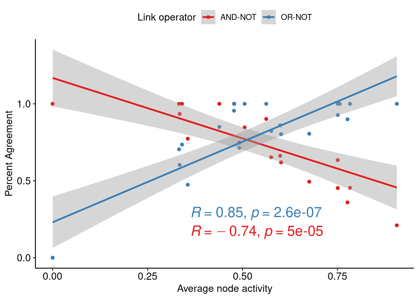

Figure 19: Correlation between parameterization-state agreement and average node activity in the CASCADE 1.0 models