MDA-MB-468 Model Analysis
This chapter includes the ensemble model analysis performed on the models
generated by the Gitsbe module when running the DrugLogics computational
pipeline for finding synergistic drug combinations (drug pairs). All these
models were trained towards a specific steady state signaling pattern that was
derived based on input data (gene expression, CNV) for the MDA-MB-468 cell line,
(Breast adenocarcinoma, a breast cancer), the use of the PARADIGM software
(Vaske et al. 2010) and a topology that was build for simulating a cancer cell fate decision network.
The input for the simulations and the output data are in the cell-lines-2500
directory (the 2500 number denotes the number of simulations executed). The
analysis will be presented step by step in the sections below.
Input
We will define the name of the cell line which must match the name of the
directory that has the input files inside the cell-lines-2500 directory. Our
analysis in this chapter will be done on the data for the MDA-MB-468 cell line:
Three inputs are used in this analysis:
- The model_predictions file which has for each model the prediction for each drug combination tested (0 = no synergy predicted, 1 = synergy predicted, NA = couldn’t find stable states in either the drug combination inhibited model or in any of the two single-drug inhibited models)
- The observed_synergies file which lists the drug combinations that were observed as synergistic for the particular cell line.
- The models directory, which is the same as the models directory produced
by
Gitsbeand has one.gitsbefile per model that includes this info:- The stable state of the boolean model. Note that a model can have 1
stable state or none in our simulations - but the models used in this analysis
have been selected through a genetic evolution algorithm in
Gitsbeand so in the end, only those with 1 stable state have higher fitness values and remain in the later generations. Higher fitness here means a better match of a model’s stable state to the cell line derived steady state (a perfect match would result in a fitness of 1) - The boolean equations of the model
- The stable state of the boolean model. Note that a model can have 1
stable state or none in our simulations - but the models used in this analysis
have been selected through a genetic evolution algorithm in
models.stable.state.file = paste0(data.dir, "models_stable_state")
observed.synergies.file  = paste0(data.dir, "observed_synergies")
model.predictions.file   = paste0(data.dir, "model_predictions")
models.equations.file    = paste0(data.dir, "models_equations")
models.dir = paste0(data.dir, "models")
Now, we parse the data into proper R objects. First the synergy predictions per model:
model.predictions = get_model_predictions(model.predictions.file)

# Example: first model's synergy predictions (first 12 drug combinations)
pretty_print_vector_names_and_values(model.predictions[1,], n = 12)
5Z-AK: 0, 5Z-BI: 0, 5Z-CT: 0, 5Z-PD: 1, 5Z-PI: 0, 5Z-PK: 0, 5Z-JN: 0, 5Z-D1: 0, 5Z-60: 0, 5Z-SB: 0, 5Z-RU: 0, 5Z-D4: 0
So, the model.predictions object has the models as rows and each column is a
different drug combination that was tested in our simulations.
drug.combinations.tested = colnames(model.predictions)
models                   = rownames(model.predictions)
nodes                    = get_node_names(models.dir)

number.of.drug.comb.tested = length(drug.combinations.tested)
number.of.models           = length(models)
number.of.nodes            = length(nodes)

print_model_and_drug_stats(number.of.drug.comb.tested, number.of.models,
                           number.of.nodes, html.output = TRUE)
Drug combinations tested: 153
Number of models: 7500
Number of nodes: 139
Next, we get the full stable state and the equations per model:
models.stable.state = as.matrix(
  read.table(file = models.stable.state.file, check.names = FALSE)
)

# Example: first model's stable state (first 12 nodes)
pretty_print_vector_names_and_values(models.stable.state[1,], n = 12)
MAP3K7: 1, MAP2K6: 1, MAP2K3: 1, NLK: 1, MAP3K4: 1, MAP2K4: 1, IKBKG: 1, IKBKB: 1, AKT1: 0, BRAF: 1, SMAD3: 1, DAB2IP: 1
The rows of the models.stable.state object represent the models while its
columns are the names of the nodes (proteins, genes, etc.) of the cancer cell
network under study. So, each model has one stable state which means that in
every model, the nodes in the network have reached a state of either 0
(inhibition) or 1 (activation).
models.equations = as.matrix(
  read.table(file = models.equations.file, check.names = FALSE)
)

# Example: first model's link operators (first 12 nodes)
pretty_print_vector_names_and_values(models.equations[1,], n = 12)
MAP3K4: 1, MAP2K4: 0, IKBKB: 1, AKT1: 0, SMAD3: 1, GSK3B: 1, RAF1: 1, GAB2: 1, CTNNB1: 0, NR3C1: 1, CREB1: 0, RAC1: 1
For the models.equations, if we look at a specific row (a model so to speak),
the columns (node names) correspond to the targets of regulation (and the
network has been built so that every node is a target - i.e. it has other
nodes activating and/or inhibiting it). The general form of a boolean equation
is:
general.equation =
  "Target *= (Activator OR Activator OR...) AND NOT (Inhibitor OR Inhibitor OR...)"
pretty_print_bold_string(general.equation)
Target *= (Activator OR Activator OR…) AND NOT (Inhibitor OR Inhibitor OR…)
The difference between the models’ boolean equations is the link operator
(OR NOT/AND NOT) which has been mutated (changed) through the evolutionary
process of the genetic algorithm in Gitsbe. For example, if a model has for
the column ERK_f (of the models.equations object) a value of 1, the correspoding
equation is: ERK_f *= (MEK_f) OR NOT ((DUSP6) OR PPP1CA). A value of 0 would
correspond to the same equation but having AND NOT as the link operator:
ERK_f *= (MEK_f) AND NOT ((DUSP6) OR PPP1CA). Note that the equations that do
not have link operators (meaning that they are the same for every model) are
discarded (so less columns in this dataset) since in a later section we study only
the equations whose link operators differentiate between the models.
Lastly, the synergies observed for this particular cell line are:
observed.synergies = get_observed_synergies(
  observed.synergies.file, drug.combinations.tested)
number.of.observed.synergies = length(observed.synergies)

pretty_print_vector_values(observed.synergies,
                           vector.values.str = "observed synergies")
14 observed synergies: AK-BI, JN-D1, PI-D1, PI-D4, BI-JN, PI-JN, BI-P5, D1-P5, G4-P5, PD-P5, PI-P5, AK-PI, BI-PI, CT-PI
Performance Statistics
It will be interesting to know the percentage of the above observed synergies that were actually predicted by at least one of the models (there might be combinations that no model in our dataset could predict): combinations that no model in our dataset could predict):
# Split model.predictions to positive and negative results
observed.model.predictions =
  get_observed_model_predictions(model.predictions, observed.synergies)
unobserved.model.predictions =
  get_unobserved_model_predictions(model.predictions, observed.synergies)

stopifnot(ncol(observed.model.predictions)
          + ncol(unobserved.model.predictions) == number.of.drug.comb.tested)

number.of.models.per.observed.synergy =
  colSums(observed.model.predictions, na.rm = TRUE)
predicted.synergies = names(which(number.of.models.per.observed.synergy > 0))

# predicted synergies is a subset of the observed (positive) ones
stopifnot(all(predicted.synergies %in% observed.synergies))5 predicted synergies: BI-PI, PI-JN, PI-D1, JN-D1, D1-P5
predicted.synergies.percentage = 100 * length(predicted.synergies) /
                    number.of.observed.synergies
pretty_print_string(paste0("Percentage of True Positive predicted synergies: ",
                    specify_decimal(predicted.synergies.percentage, 2), "%"))
Percentage of True Positive predicted synergies: 35.71%
So, for this particular cell line, there were indeed observed synergies that no
model could predict (e.g.
AK-BI,
AK-PI).
Next, we would like to know the maximum
number of observed synergies predicted by one model alone - can one model by itself
predict all the true positive synergies predicted by all the models together or
do we need many models to capture this diverse synergy landscape? To do that, we
go even further and count the number of models that predict a specific set of
observed synergies for every possible combination subset of the predicted.synergies
object:
# Find the number of predictive models for every synergy subset
synergy.subset.stats = get_synergy_subset_stats(observed.model.predictions, predicted.synergies)

# Bar plot of the number of models for every possible observed synergy combination set
# Tweak the threshold.for.subset.removal and bottom.margin as desired
make_barplot_on_synergy_subset_stats(synergy.subset.stats,
                                     threshold.for.subset.removal = 1,
                                     bottom.margin = 9, cell.line)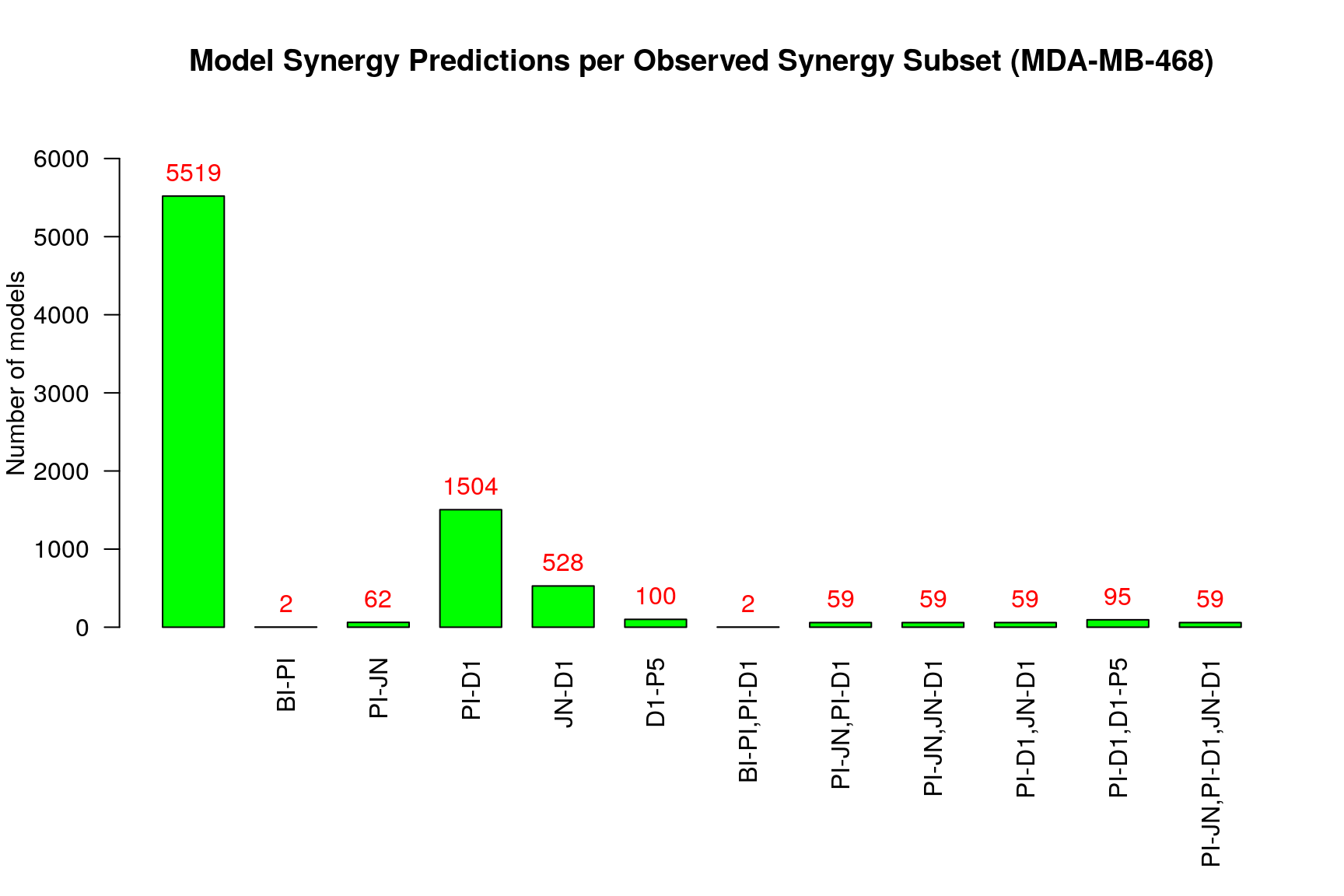
From the above figure (where we excluded sets of synergies that were predicted
by no model by setting the threshold.for.subset.removal value to 1) we observe
that:
- More than half of the models predict none of the observed synergies
- The
PI-D1synergy is the most common predicted synergy for the rest of the models
Next we calculate the maximum number of correctly predicted synergies (\(TP\) - True Positives) per model:
# Count the predictions of the observed synergies per model (TP)
models.synergies.tp = calculate_models_synergies_tp(observed.model.predictions)
models.synergies.tp.stats = table(models.synergies.tp)

# Bar plot of number of models vs correctly predicted synergies
make_barplot_on_models_stats(models.synergies.tp.stats, cell.line,
                             title = "True Positive Synergy Predictions",
                             xlab = "Number of maximum correctly predicted synergies",
                             ylab = "Number of models")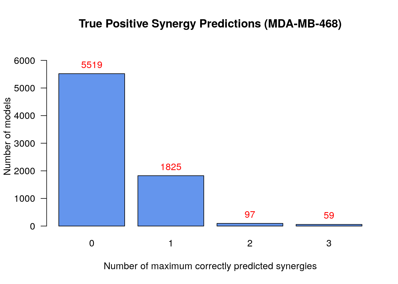
To summarize:
- There were 59
models that predicted 3
synergies - the set
PI-JN,PI-D1,JN-D1- which is the maximum number of predicted synergies by an individual model - No model could predict all 5 of the total predicted synergies
The power of the ensemble model approach lies in the fact that (as
we saw from the above figures) even though we may not have individual super models
that can predict many observed drug combinations, there are many that predict
at least one and which will be used by the drug response analysis module
(Drabme) to better infer the synergistic drug combinations. It goes without
saying though, that the existance of models that could predict more than a
handful of synergies would be beneficial for any approach that performs drug
response analysis on a multitude of models.
Biomarker analysis
Intro-Methods
Now, we want to investigate and find possible important nodes - biomarkers - whose activity state either distinguishes good performance models from less performant ones (in terms of a performance metric - e.g. the true positive synergies predicted) or makes some models predict a specific synergy compared to others that can’t (but could predict other synergies). So, we devised two strategies to split the models in our disposal to good and bad ones (but not necessarily all of them), the demarcation line being either a performance metric (the number of \(TP\) or the Matthews Correlation Coefficient score) or the prediction or not of a specific synergy. Then, for each group of models (labeled as either good or bad) we find the average activity state of every node in the network (value between 0 and 1) and then we compute the average state difference for each node between the two groups: \(\forall i\in nodes,mean(state_i)_{good} - mean(state_i)_{bad}\). Our hypothesis is that if the absolute value of these average differences are larger than a user-defined threshold (e.g. 0.7) for a small number of nodes (the less the better) while for the rest of the nodes they remain close to zero, then the former nodes are considered the most important since they define the difference between the average bad model and the average good one in that particular case study. We will also deploy a network visualization method to observe these average differences.
True Positives-based analysis
Using our first strategy, we will split the models based on the number of true
positive predictions. For example, the bad models will be the ones that
predicted 0 \(TP\) synergies whereas the good models will be the ones that predicted
2 \(TP\) (we will denote the grouping as \((0,2)\)). This particular classification
strategy will be used for every possible combination of the number of \(TP\) as
given by the models.synergies.tp.stats object and the density estimation of the
nodes’ average state differences in each case will be ploted in a common graph:
diff.tp.results = get_avg_activity_diff_mat_based_on_tp_predictions(
  models, models.synergies.tp, models.stable.state)

tp.densities = apply(abs(diff.tp.results), 1, density)
make_multiple_density_plot(tp.densities, legend.title = "True Positives",
                           x.axis.label = "Activity state (absolute difference value)",
                           title = "Density Estimation for the Average State Difference")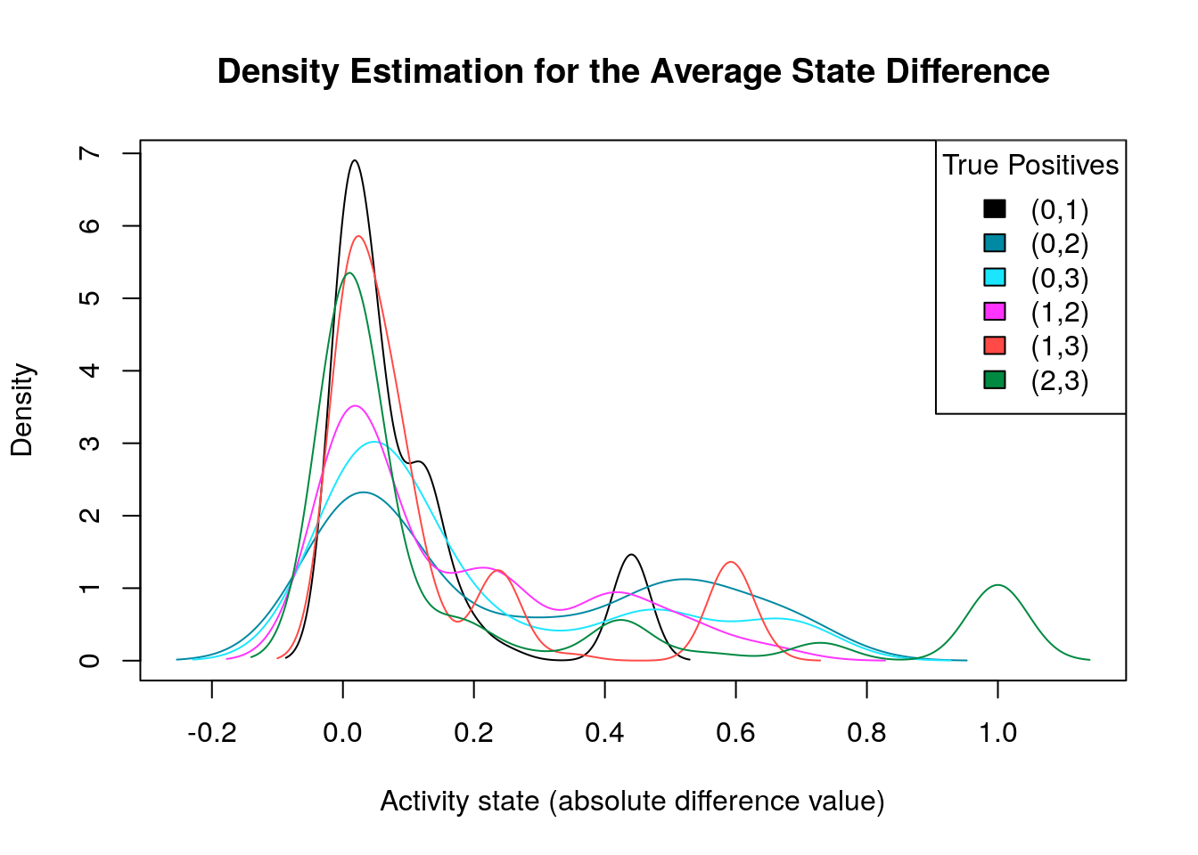
What we are actually looking for is density plots that are largely skewed to the right (so the average absolute differences of these nodes are close to zero) while there are a few areas of non-zero densities which are as close to 1 as possible. So, from the above graph, the density plots that fit this description are the ones marked as \((1,3)\) and \((2,3)\). We will visualize the nodes’ average state differences in a network graph (Csardi and Nepusz 2006), where the color of each node will denote how much more inhibited or active that node is, in the average good model vs the average bad one. The color of the edges will denote activation (green) or inhibition (red). We first build the network from the node topology (edge list):
parent.dir = get_parent_dir(data.dir)
topology.file = paste0(parent.dir, "/topology")
coordinates.file = paste0(parent.dir, "/network_xy_coordinates")

net = construct_network(topology.file, models.dir)

# a static layout for plotting the same network always (igraph)
# nice.layout = layout_nicely(net)
nice.layout = as.matrix(read.table(coordinates.file))
In the next colored graphs we can identify the important nodes whose activity state can influence the true positive prediction performance (from 0 true positive synergies to a total of 3):
plot_avg_state_diff_graph(net, diff.tp.results["(0,3)",], layout = nice.layout,
             title = "Bad models (0 TP) vs Good models (3 TP)")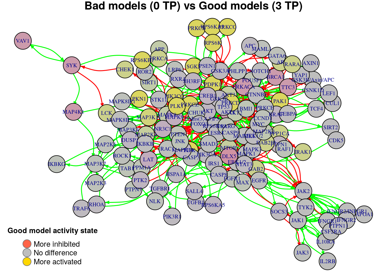
plot_avg_state_diff_graph(net, diff.tp.results["(1,3)",], layout = nice.layout,
             title = "Bad models (1 TP) vs Good models (3 TP)")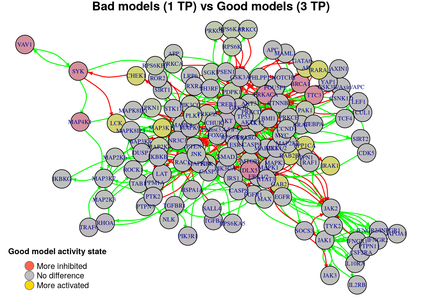
plot_avg_state_diff_graph(net, diff.tp.results["(2,3)",], layout = nice.layout,
             title = "Bad models (2 TP) vs Good models (3 TP)")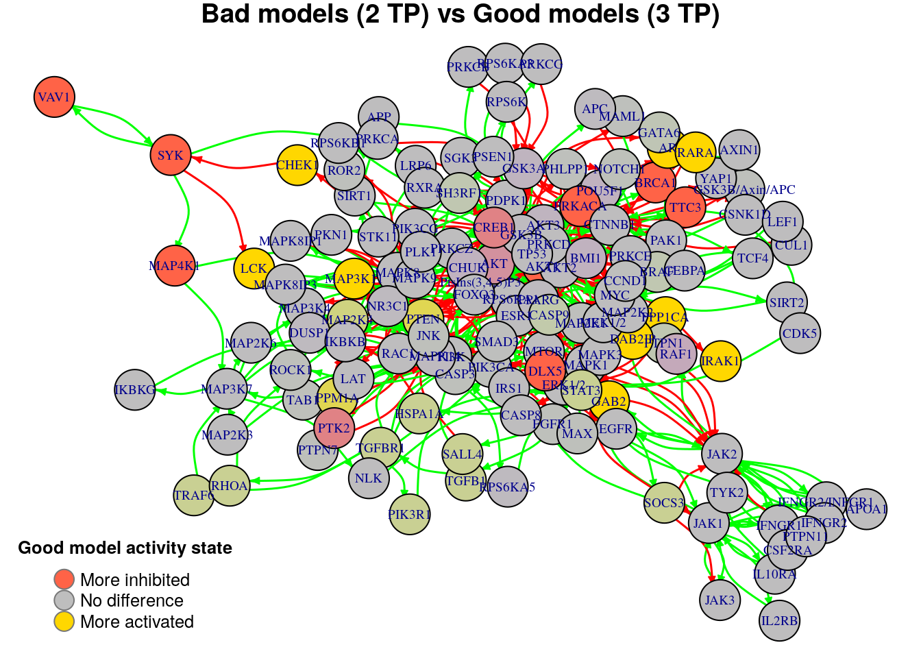
We will now list the important nodes that affect the models’ prediction performance with regards to the number of true positive synergies that they predict. Comparing the graphs above, we observe that there exist common nodes that maintain the same significant influence in all of the graphs. We set the threshold for the absolute significance level in average state differences to \(0.7\). A node will be marked as a biomarker (active or inhibited) if its activity state difference surpassed the aforementioned threshold (positively or negatively) for any of the tested groups (e.g. 2 \(TP\) vs 3 \(TP\)). So, the nodes that have to be in a more active state are:
biomarkers.tp.active = get_biomarkers_per_type(
  diff.tp.results, threshold = 0.7, type = "positive"
)
pretty_print_vector_values(biomarkers.tp.active)
11 nodes: DAB2IP, PPP1CA, AR, CHEK1, GAB2, RARA, IRAK1, MAP3K11, PTEN, PPM1A, LCK
Also, the nodes that have to be in a more inhibited state are:
biomarkers.tp.inhibited = get_biomarkers_per_type(
  diff.tp.results, threshold = 0.7, type = "negative"
)
pretty_print_vector_values(biomarkers.tp.inhibited)
10 nodes: AKT1, BRCA1, DLX5, PRKACA, TTC3, CREB1, PTK2, SYK, MAP4K1, VAV1
We check if there are nodes found by our method as biomarkers in both active and inhibited states:
No common nodes
MCC classification-based analysis
The previous method to split the models based on the number of true positive predictions is a good metric for absolute performance but a very restricted one since it ignores the other values of the confusion matrix for each model (true negatives, false positives, false negatives). Also, since our dataset is imbalanced in the sense that out of the total drug combinations tested only a few of them are observed as synergistic (and in a hypothetical larger drug screening evaluation it will be even less true positives) we will now devise a method to split the models into different performance categories based on the value of the Matthews Correlation Coefficient (MCC) score which takes into account the balance ratios of all the four confusion matrix values:
# Calculate Matthews Correlation Coefficient (MCC) for every model
models.mcc = calculate_models_mcc(observed.model.predictions,
                                  unobserved.model.predictions,
                                  number.of.drug.comb.tested)

models.mcc.stats = table(models.mcc, useNA = "ifany")

make_barplot_on_models_stats(models.mcc.stats, cell.line, title = "MCC scores",
                             xlab = "MCC value", ylab = "Number of models",
                             cont.values = TRUE, threshold = 10)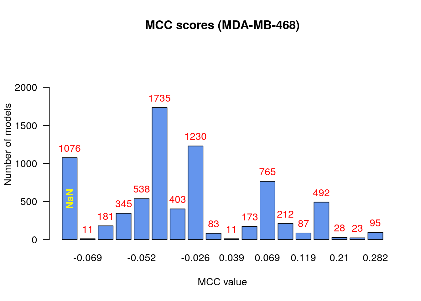
Note that for presentation purposes in the figure above, we pruned some MCC-bars with lower model frequency values. We observe that:
- There are no relatively bad models (MCC values close to -1)
- Most of the models (exluding the
NaNcategory) perform a little better than random prediction (\(MCC>0\)) - There are models that had
NaNvalue for the MCC score
Given the MCC formula:
\(MCC = (TP\cdot TN - FP\cdot FN)/\sqrt{(TP+FP) * (TP+FN) * (TN+FP) * (TN+FN)}\),
we can see that the MCC value can be NaN because of zero devision. Two of the
four values in the denominator represent the number of positive \((TP+FN)\) and
negative \((TN+FP)\) observations which are non-zero for every model, since they
correspond to the observed and non-obsered synergies in each case.
The case where both \(TN\) and \(FN\) are zero is rare (if non-existent)
because of the imbalanced dataset (large proportion of negatives) and the reason
that logical models which report no negatives means that they should find
fixpoint attractors for every possible drug combination perturbation which also
is extremely unlikely. We can actually see that the NaN are produced by models
that have both TP and FP equal to zero:
models.synergies.fp = calculate_models_synergies_fp(unobserved.model.predictions)
pretty_print_string(sum(models.synergies.tp + models.synergies.fp == 0))
1076
Since these models could intentify no synergies (either correctly or
wrongly), we decided to put them as the lowest performant category in our
MCC-based analysis. To classify the models based on their MCC score (which takes
values in the \([-1, 1]\) interval, NaN values excluded), we will perform a
univariate k-means clustering to split the previously found MCC values to
different classes (Wang and Song 2011). The MCC classification is presented with a histogram:
num.of.classes = 5
mcc.class.ids = 1:num.of.classes

models.mcc.no.nan = models.mcc[!is.nan(models.mcc)]
models.mcc.no.nan.sorted = sort(models.mcc.no.nan)

# find the clusters
res = Ckmeans.1d.dp(x = models.mcc.no.nan.sorted, k = num.of.classes)
models.cluster.ids = res$cluster

plot_mcc_classes_hist(models.mcc.no.nan.sorted, models.cluster.ids,
                      num.of.classes, mcc.class.ids)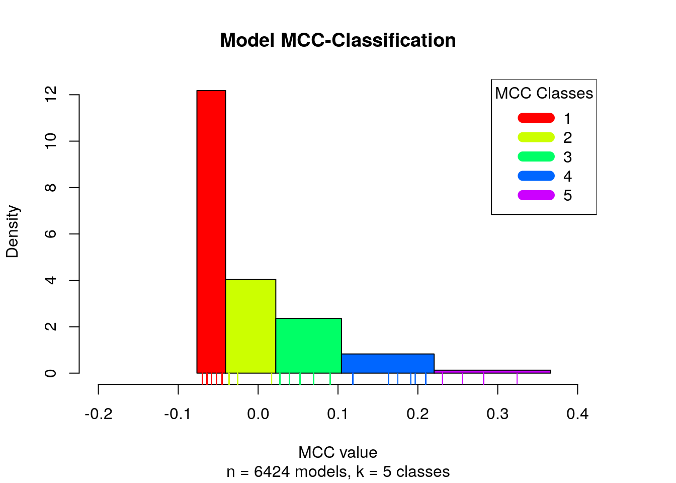
Note that in total we have 6 MCC classes, since the NaN MCC values constitute
a class on its own.
Following our first strategy, we will split the models based on the MCC
performance metric score. For example, the bad models will be the ones that
had a NaN MCC score \((TP+FP = 0)\) whereas the good models will be the ones that
had an MCC score belonging to the first MCC class as seen in the histogram above.
This particular classification strategy will be used for every possible combination
of the MCC classes and the density estimation of the nodes’ average state
differences in each case will be ploted in a common graph:
# add NaN class (if applicable)
if (sum(is.nan(models.mcc)) > 0) {
  mcc.class.ids = append(mcc.class.ids, values = NaN, after = 0)
}

mcc.class.id.comb = t(combn(1:length(mcc.class.ids), 2))

diff.mcc.results = apply(mcc.class.id.comb, 1, function(comb) {
  return(get_avg_activity_diff_based_on_mcc_clustering(
          models.mcc, models.stable.state,
          mcc.class.ids, models.cluster.ids,
          class.id.low = comb[1], class.id.high = comb[2]))
})

mcc.classes.comb.names = apply(mcc.class.id.comb, 1, function(comb) {
  return(paste0("(", mcc.class.ids[comb[1]], ",", mcc.class.ids[comb[2]], ")"))
})

colnames(diff.mcc.results) = mcc.classes.comb.names
diff.mcc.results = t(diff.mcc.results)

mcc.densities = apply(abs(diff.mcc.results), 1, density)
make_multiple_density_plot(mcc.densities, legend.title = "MCC classes",
                           x.axis.label = "Activity state (absolute difference value)",
                           title = "Density Estimation for the Average State Difference",
                           legend.size = 0.7)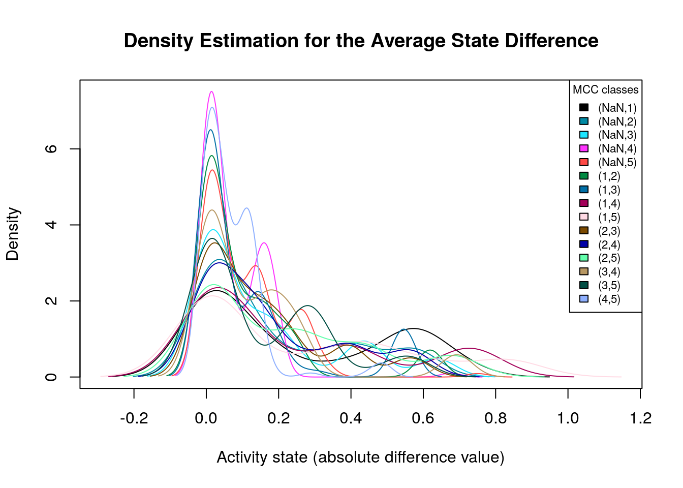
Many of the density plots above are of interest to us, since they are right skewed. Next, we visualize the average state differences with our network coloring method for 2 of the above cases, in order to identify the important nodes whose activity state can influence the prediction performance based on the MCC classification:
plot_avg_state_diff_graph(net, diff.mcc.results["(NaN,4)",], layout = nice.layout,
             title = "Bad models (MCC Class: NaN) vs Good models (MCC Class: 4)")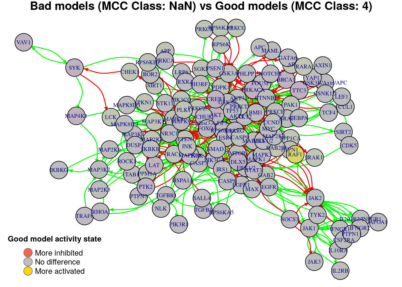
plot_avg_state_diff_graph(net, diff.mcc.results["(1,4)",], layout = nice.layout,
             title = "Bad models (MCC Class: 1) vs Good models (MCC Class: 4)")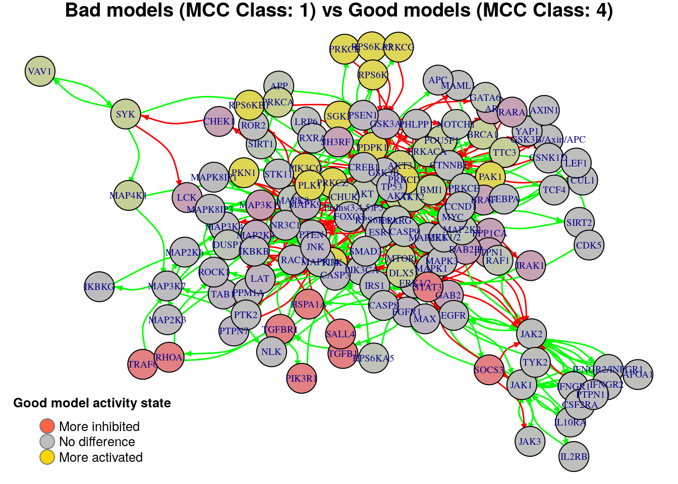
We will now list the important nodes that affect the models’ prediction
performance with regards to their MCC classification, using the same method
as in the True Positives-based analysis section. First, the nodes that have to
be in a more active state:
biomarkers.mcc.active = get_biomarkers_per_type(
  diff.mcc.results, threshold = 0.7, type = "positive"
)
pretty_print_vector_values(biomarkers.mcc.active)
16 nodes: RAF1, PtsIns(3,4,5)P3, PI3K, PIK3CG, RPS6K, PDPK1, RPS6KB1, PLK1, RPS6KA3, PRKCD, PRKCZ, PKN1, SGK3, PRKCB, PRKCG, PAK1
Secondly, the nodes that have to be in a more inhibited state:
biomarkers.mcc.inhibited = get_biomarkers_per_type(
  diff.mcc.results, threshold = 0.7, type = "negative"
)
pretty_print_vector_values(biomarkers.mcc.inhibited)
9 nodes: STAT3, SOCS3, TGFB1, HSPA1A, SALL4, TGFBR1, TRAF6, RHOA, PIK3R1
We check if there are nodes found by our method as biomarkers in both active and inhibited states:
No common nodes
Equation-based analysis
It will be interesting to see the different patterns in the form of the boolean
equations (regarding the mutation of the link operator as mentioned in the Input
section) when comparing higher performance models vs the low performant ones. We
could also check if any of the biomarkers found above relate to a different link
operator on average between models with different performance characteristics
(e.g. higher predictive models should have the OR NOT as the link operator in
a boolean equation where a specific biomarker is the regulation target) or if they
constitute targets of exclusively activating nodes or inhibiting ones (an equation
with no link operator).
The performance metric we will first use to sort the models is the number of true
positive predictions. We will now illustrate the heatmap of the models.equations
object raw-order by the number of \(TP\) predictions:
# order based on number of true positives
models.synergies.tp.sorted = sort(models.synergies.tp)
models.sorted = names(models.synergies.tp.sorted)
models.equations.sorted = models.equations[models.sorted, ]

# coloring
eq.link.colors = c("red", "lightyellow")
eq.link.col.fun = colorRamp2(breaks = c(0, 1), colors = eq.link.colors)
tp.values = sort(unique(models.synergies.tp))
tp.col.fun = colorRamp2(breaks = c(min(tp.values), max(tp.values)),
                         colors = c("red", "green"))

# color biomarker names in the heatmap
bottom.nodes.colors = rep("black", length(colnames(models.equations.sorted)))
names(bottom.nodes.colors) = colnames(models.equations.sorted)
bottom.nodes.colors[names(bottom.nodes.colors) %in%
                    biomarkers.perf.active] = "blue"
bottom.nodes.colors[names(bottom.nodes.colors) %in%
                    biomarkers.perf.inhibited] = "magenta"

# define the TP color bar
tp.annot = rowAnnotation(
  tp = anno_simple(x = models.synergies.tp.sorted, col = tp.col.fun),
  show_annotation_name = FALSE)

heatmap.eq =
  Heatmap(matrix = models.equations.sorted, column_title = "Models Link Operators",
    column_title_gp = gpar(fontsize = 20), row_title = "Models (TP sorted)",
    cluster_rows = FALSE, show_row_names = FALSE, show_heatmap_legend = FALSE,
    column_dend_height = unit(1, "inches"), col = eq.link.col.fun,
    column_names_gp = gpar(fontsize = 9, col = bottom.nodes.colors),
    left_annotation = tp.annot,
    use_raster = TRUE, raster_device = "png", raster_quality = 10)

# define the 3 legends
link.op.legend = Legend(title = "Link Operator", labels = c("AND", "OR"),
                        legend_gp = gpar(fill = eq.link.colors))
tp.values = min(tp.values):max(tp.values) # maybe some integers are missing
tp.legend = Legend(at = tp.values, title = "TP",
                   legend_gp = gpar(fill = tp.col.fun(tp.values)))
biomarkers.legend = Legend(title = "Biomarkers", labels = c("Inhibited", "Active"),
                           legend_gp = gpar(fill = c("magenta", "blue")))
legend.list = packLegend(link.op.legend, tp.legend, biomarkers.legend,
                         direction = "vertical")

draw(heatmap.eq, annotation_legend_list = legend.list,
annotation_legend_side = "right")-1.png)
In the heatmap above, an equation whose link operator is AND NOT is represented
with red color while an OR NOT link operator is represented with light yellow color.
The targets whose equations do not have a link operator are not represented.
The rows are ordered by the number of true positive predictions (ascending).
We have colored the names of the network nodes that were also found as biomarkers
(green color is used for the active biomarkers and red color for the inhibited
biomarkers). We observe that:
- Most of the biomarkers are nodes that do not have both activators and inhibitors and so are absent from the above heatmap
- There doesn’t seem to exist a pattern between the models’ link operators and their corresponding performance (at least not for all of the nodes) when using the true positive predictions as a classifier for the models
- There exist a lot of target nodes that need to have the
OR NOTlink operator in their respective boolean equation in order for the corresponding logical model to show a higher number of true positive predictions. By assigning theOR NOTlink operator to a target’s boolean regulation equation, we allow more flexibility to the target’s output active result state - meaning that the inhibitors play less role and the output state has a higher probability of being active - compared to assigning theAND NOTlink operator to the equation
We will also illustrate the heatmap of the models.equations object raw-order
by the MCC score which is a better performance classifier. Models who had a NaN
MCC score will be again placed in the lower performant category:
# order based on the MCC value
models.mcc.sorted = sort(models.mcc, na.last = FALSE)
models.sorted = names(models.mcc.sorted)
models.equations.sorted = models.equations[models.sorted, ]

# coloring
mcc.col.fun =
  colorRamp2(breaks = c(min(models.mcc.no.nan),
                        max(models.mcc.no.nan)), colors = c("red", "green"))

# define the MCC color bar
mcc.annot = rowAnnotation(
  mcc = anno_simple(x = models.mcc.sorted, col = mcc.col.fun, na_col = "black"),
  show_annotation_name = FALSE)

heatmap.eq =
  Heatmap(matrix = models.equations.sorted, column_title = "Models Link Operators",
    column_title_gp = gpar(fontsize = 20), row_title = "Models (MCC sorted)",
    cluster_rows = FALSE, show_row_names = FALSE, show_heatmap_legend = FALSE,
    column_dend_height = unit(1, "inches"), col = eq.link.col.fun,
    column_names_gp = gpar(fontsize = 9, col = bottom.nodes.colors),
    left_annotation = mcc.annot,
    use_raster = TRUE, raster_device = "png", raster_quality = 10)

# define the 4 legends
link.op.legend = Legend(title = "Link Operator", labels = c("AND", "OR"),
                        legend_gp = gpar(fill = eq.link.colors))
mcc.legend = Legend(title = "MCC", col_fun = mcc.col.fun)
na.legend = Legend(labels = "NA", legend_gp = gpar(fill = "black"))
biomarkers.legend = Legend(title = "Biomarkers", labels = c("Inhibited", "Active"),
                           legend_gp = gpar(fill = c("magenta", "blue")))
legend.list = packLegend(link.op.legend, mcc.legend, na.legend, biomarkers.legend,
                         direction = "vertical")

draw(heatmap.eq, annotation_legend_list = legend.list,
annotation_legend_side = "right")-1.png)
In the MCC-ordered heatmap above we observe that there is better correlation
between the boolean equations’ link operators and the performance of a model
compared to the \(TP\) classification. For example, the biomarkers STAT3 and
RAF1 show distinguished patterns for the higher performance models (use of
AND NOT and OR NOT link operators respectively) when the models are sorted
by the MCC score.
Synergy-prediction based analysis
We will now use the second strategy to split the models, based on whether
they predict a specific observed synergy or not. This will allow us
to find biomarkers that affect the prediction of a specific synergy.
For example, the good models could be the ones that predicted the hypothetical
synergy A-B while the bad models all the rest that identified the particular
combination as non-synergistic.
In another case scenario, the good models could be those that predicted a
triple synergy set A-B,C-D,A-C, while the bad models could be the ones
that predicted the double synergy subset A-B,C-D (excluding the common models
that predicted both the triple synergy set and subsequently its given subset).
In such a case scenario, we want to find out which nodes are responsible for making
the good models predict the extra synergy - in this hypothetical case the
synergy A-C - demonstrating thus better model performance. Note that the models
selected in each case as good or bad, could have predicted other synergies as well
(correctly as \(TP\) or wrongly as \(FP\)) which means that the biomarker selection
method could be somewhat innacurate, since we can’t really know the prediction of
which extra synergy or synergies the biomarkers’ state affected. To account for
this, we label as good models those that predict large synergy sets (so fewer
models) which capture almost all the true positive predictions and also minimize
the possible extra different synergies predicted by models of the same classification
category (e.g. the good models).
Starting with the first model classification method (prediction vs non-prediction of a particular synergy), we generate the density distribution of the nodes’ average state differences between the good and bad models for each predicted synergy:
diff.predicted.synergies.results =
  sapply(predicted.synergies, function(drug.comb) {
    get_avg_activity_diff_based_on_specific_synergy_prediction(
      model.predictions, models.stable.state, drug.comb)
  })
diff.predicted.synergies.results = t(diff.predicted.synergies.results)

densities = apply(abs(diff.predicted.synergies.results), 1, density)
make_multiple_density_plot(densities, legend.title = "Predicted Synergies",
                           x.axis.label = "Activity state (absolute difference value)",
                           title = "Density Estimation for the Average State Difference")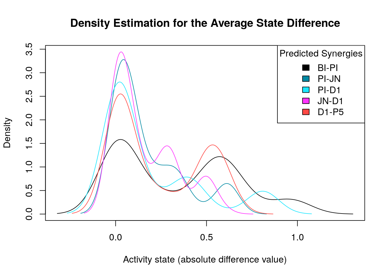
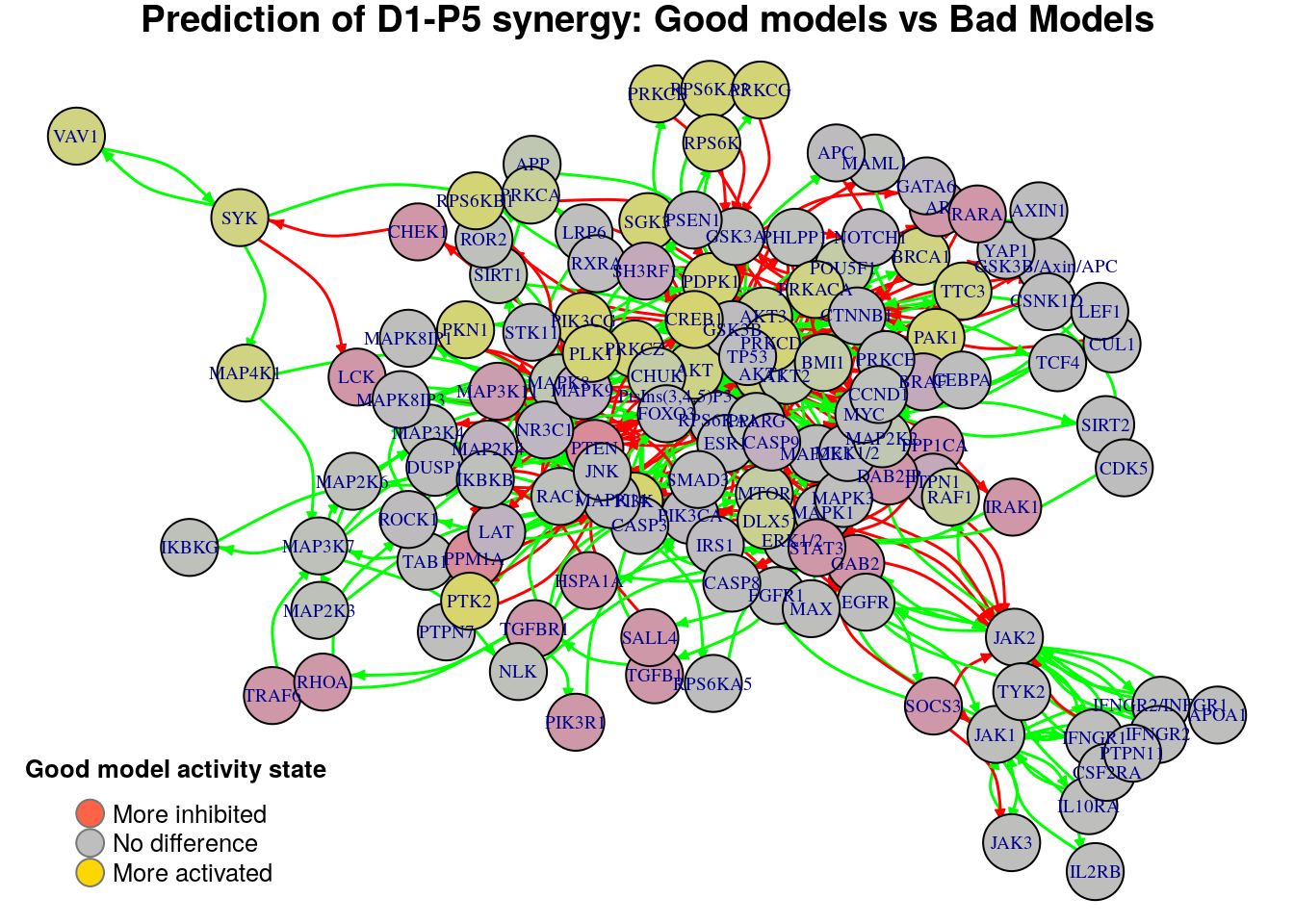
Next, we will plot the biomarkers with the network visualization method (for all predicted synergies) and output the respective biomarkers in each case. The biomarker results for each predicted synergy will be stored for further comparison with the results from the other cell lines.
threshold = 0.7
for (drug.comb in predicted.synergies) {
  diff = diff.predicted.synergies.results[drug.comb, ]

  biomarkers.active = diff[diff > threshold]
  biomarkers.inhibited = diff[diff < -threshold]

  save_vector_to_file(vector = biomarkers.active, file = paste0(
    biomarkers.dir, drug.comb, "_biomarkers_active"), with.row.names = TRUE)
  save_vector_to_file(vector = biomarkers.inhibited, file = paste0(
    biomarkers.dir, drug.comb, "_biomarkers_inhibited"), with.row.names = TRUE)
}
threshold = 0.7
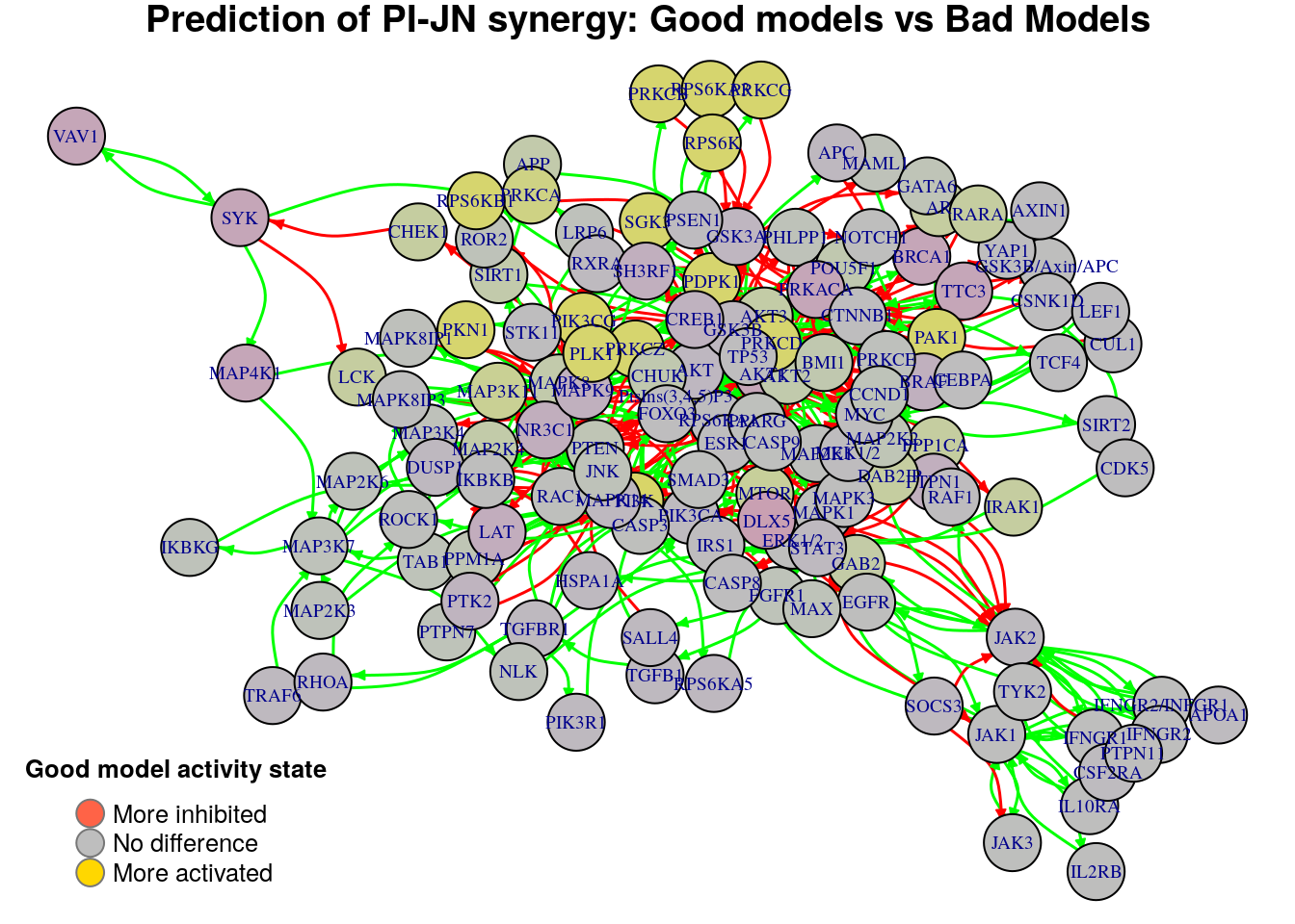
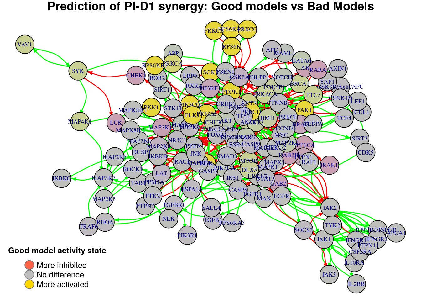
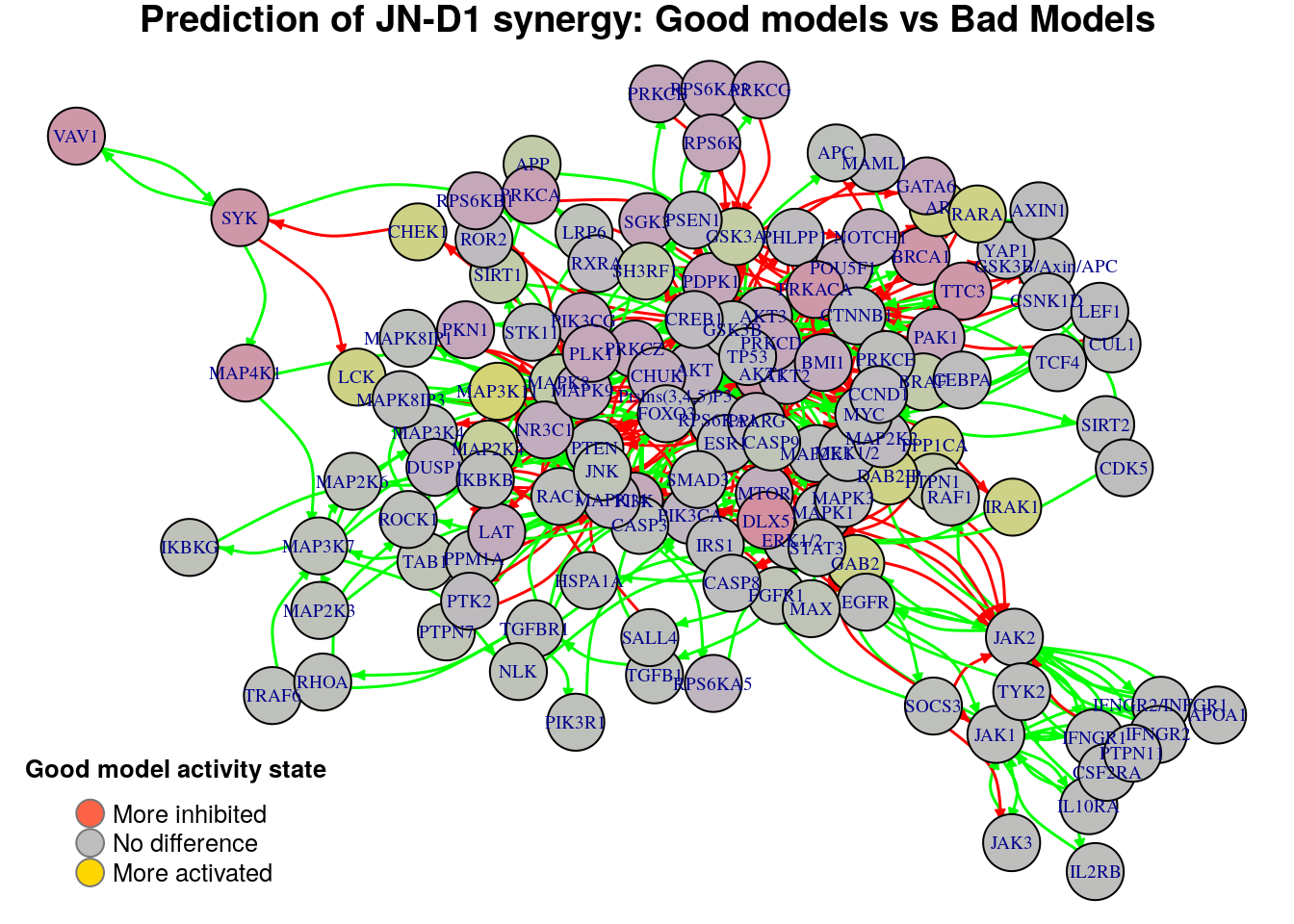
for (drug.comb in predicted.synergies) {
title.text = paste0("Prediction of ", drug.comb,
" synergy: Good models vs Bad Models")
diff = diff.predicted.synergies.results[drug.comb, ]
plot_avg_state_diff_graph(net, diff, layout = nice.layout, title = title.text)
}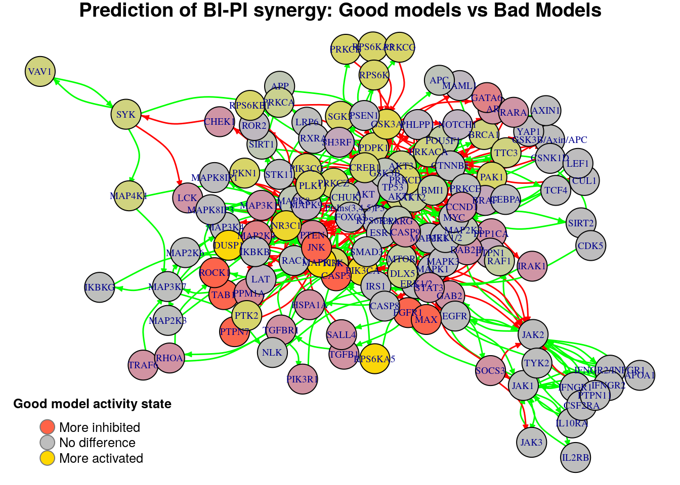
Biomarkers for BI-PI synergy prediction
Active biomarkers
6 nodes: NR3C1, GSK3A, MAPK14, RPS6KA5, DUSP1, PIK3CA
Inhibited biomarkers
9 nodes: MAP2K4, FGFR1, TAB1, CASP3, PTPN7, MAX, GATA6, JNK, ROCK1
Biomarkers for PI-JN synergy prediction
Active biomarkers
0 nodes:
Inhibited biomarkers
0 nodes:
Biomarkers for PI-D1 synergy prediction
Active biomarkers
15 nodes: PtsIns(3,4,5)P3, PI3K, PIK3CG, RPS6K, PDPK1, RPS6KB1, PLK1, RPS6KA3, PRKCD, PRKCZ, PKN1, SGK3, PRKCB, PRKCG, PAK1
Inhibited biomarkers
0 nodes:
Biomarkers for JN-D1 synergy prediction
Active biomarkers
0 nodes:
Inhibited biomarkers
0 nodes:
Biomarkers for D1-P5 synergy prediction
Active biomarkers
0 nodes:
Inhibited biomarkers
0 nodes:
We notice that for some predicted synergies the above method identified zero biomarkers. We will now study cases where the main goal is the better identification and/or refinement of the biomarkers responsible for allowing the models to predict one extra synergy from a specific synergy set. If we find biomarkers for a predicted synergy using this strategy, we compare them to the ones already found with the previous method and if none of them is common we just add the new ones to the list of biomarkers for that specific synergy. On the other hand, if the synergy-set comparison method identifies a subset of the previously found biomarkers for a specific synergy (one common node at least), we will only keep the later method’s biomarkers since we believe that the synergy-set prediction based method is more accurate at identifying biomarkers for a specific synergy because of the fewer models involved in each contrasting category which also minimizes the total false positive synergy predictions taken into account. Note that if the second method finds even more biomarkers than the first, we have the option to prune the end result to only the common biomarkers between the two methods.
We will focus our analysis on the predicted synergies PI-JN, JN-D1, D1-P5,
PI-D1 and BI-PI.
Synergy-set prediction based analysis
PI-JN synergy
The first use case will contrast the models that predicted the synergy set
PI-JN,JN-D1 vs the models that predicted the single synergy JN-D1 as well
as the models that predicted the synergy set PI-JN,PI-D1 vs the models that
predicted the single synergy PI-D1. This will allow us to find important nodes
whose state can influence the prediction performance of a model and make it
predict the extra PI-JN synergy:
synergy.set.str.1    = "PI-JN,JN-D1"
synergy.subset.str.1 = "JN-D1"
diff.PI.JN.1 = get_avg_activity_diff_based_on_synergy_set_cmp(
  synergy.set.str.1, synergy.subset.str.1, model.predictions, models.stable.state)

synergy.set.str.2    = "PI-JN,PI-D1"
synergy.subset.str.2 = "PI-D1"
diff.PI.JN.2 = get_avg_activity_diff_based_on_synergy_set_cmp(
  synergy.set.str.2, synergy.subset.str.2, model.predictions, models.stable.state)
We now visualize the average state differences:
title.text = paste0("Good models (", synergy.set.str.1,
                    ") vs Bad Models (", synergy.subset.str.1, ")")
plot_avg_state_diff_graph(net, diff.PI.JN.1, layout = nice.layout, title = title.text)-1.png)
title.text = paste0("Good models (", synergy.set.str.2,
                    ") vs Bad Models (", synergy.subset.str.2, ")")
plot_avg_state_diff_graph(net, diff.PI.JN.2, layout = nice.layout, title = title.text)-2.png)
As we see from the above graphs, each comparison produces different biomarkers
for the PI-JN synergy. Note that with the previous method where we contrasted
the models that predict the PI-JN synergy vs those that don’t, we weren’t
able to identify not even one biomarker. We report the active biomarkers found
from the two comparisons and check whether there were any common nodes found:
biomarkers.PI.JN.active.1 = diff.PI.JN.1[diff.PI.JN.1 > threshold]
pretty_print_vector_names(biomarkers.PI.JN.active.1)
16 nodes: PtsIns(3,4,5)P3, PI3K, PIK3CG, RPS6K, PDPK1, RPS6KB1, PLK1, RPS6KA3, PRKCD, PRKCZ, PKN1, PRKCA, SGK3, PRKCB, PRKCG, PAK1
biomarkers.PI.JN.active.2 = diff.PI.JN.2[diff.PI.JN.2 > threshold]
pretty_print_vector_names(biomarkers.PI.JN.active.2)
9 nodes: DAB2IP, PPP1CA, AR, CHEK1, GAB2, RARA, IRAK1, MAP3K11, LCK
biomarkers.PI.JN.active.common.1.2 =
  get_common_names(biomarkers.PI.JN.active.1, biomarkers.PI.JN.active.2)
No common nodes
So, since there were no common active biomarkers we merged the results into one.
The inhibited biomarkers found by the two comparisons are:
biomarkers.PI.JN.inhibited.1 = diff.PI.JN.1[diff.PI.JN.1 < -threshold]
pretty_print_vector_names(biomarkers.PI.JN.inhibited.1)
0 nodes:
biomarkers.PI.JN.inhibited.2 = diff.PI.JN.2[diff.PI.JN.2 < -threshold]
pretty_print_vector_names(biomarkers.PI.JN.inhibited.2)
8 nodes: AKT1, BRCA1, DLX5, PRKACA, TTC3, SYK, MAP4K1, VAV1
Since the first comparison does not identify any inhibited biomarkers at the \(0.7\) threshold level, we use the inhibited biomarkers found from the second comparison. Lastly, we update the biomarkers for this specific synergy in the respective file:
JN-D1 synergy
The second use case will contrast the models that predicted the synergy set
PI-JN,JN-D1 vs the models that predicted the single synergy PI-JN as well
as the models that predicted the synergy set PI-D1,JN-D1 vs the models that
predicted the single synergy PI-D1. This will allow us to find important nodes
whose state can influence the prediction performance of a model and make it
predict the extra JN-D1 synergy:
synergy.set.str.1    = "PI-JN,JN-D1"
synergy.subset.str.1 = "PI-JN"
diff.JN.D1.1 = get_avg_activity_diff_based_on_synergy_set_cmp(
  synergy.set.str.1, synergy.subset.str.1, model.predictions, models.stable.state)

synergy.set.str.2    = "PI-D1,JN-D1"
synergy.subset.str.2 = "PI-D1"
diff.JN.D1.2 = get_avg_activity_diff_based_on_synergy_set_cmp(
  synergy.set.str.2, synergy.subset.str.2, model.predictions, models.stable.state)
We now visualize the average state differences:
title.text = paste0("Good models (", synergy.set.str.1,
                    ") vs Bad Models (", synergy.subset.str.1, ")")
plot_avg_state_diff_graph(net, diff.JN.D1.1, layout = nice.layout, title = title.text)-1.png)
title.text = paste0("Good models (", synergy.set.str.2,
                    ") vs Bad Models (", synergy.subset.str.2, ")")
plot_avg_state_diff_graph(net, diff.JN.D1.2, layout = nice.layout, title = title.text)-2.png)
As we see from the above graphs, each comparison produces different biomarkers
for the JN-D1 synergy. Note that with the previous method where we contrasted
the models that predict the JN-D1 synergy vs those that don’t, we weren’t able
to identify not even one biomarker. We report the active biomarkers found from the
two comparisons and check whether there were any common nodes found:
biomarkers.JN.D1.active.1 = diff.JN.D1.1[diff.JN.D1.1 > threshold]
pretty_print_vector_names(biomarkers.JN.D1.active.1)
23 nodes: GAB2, AKT3, PPARG, MAP2K2, PtsIns(3,4,5)P3, PI3K, PIK3CG, JAK2, CSF2RA, APOA1, RPS6K, PDPK1, RPS6KB1, PLK1, RPS6KA3, PRKCD, PRKCZ, PKN1, PRKCA, SGK3, PRKCB, PRKCG, PAK1
biomarkers.JN.D1.active.2 = diff.JN.D1.2[diff.JN.D1.2 > threshold]
pretty_print_vector_names(biomarkers.JN.D1.active.2)
9 nodes: DAB2IP, PPP1CA, AR, CHEK1, GAB2, RARA, IRAK1, MAP3K11, LCK
biomarkers.JN.D1.active.common.1.2 =
  get_common_names(biomarkers.JN.D1.active.1, biomarkers.JN.D1.active.2)
1 node: GAB2
biomarkers.JN.D1.active =
  c(biomarkers.JN.D1.active.1, biomarkers.JN.D1.active.2)
biomarkers.JN.D1.active =
  biomarkers.JN.D1.active[unique(names(biomarkers.JN.D1.active))]
Since there was just one common node, we merged the results and removed the duplicated node.
The inhibited biomarkers found by the two comparisons are:
biomarkers.JN.D1.inhibited.1 = diff.JN.D1.1[diff.JN.D1.1 < -threshold]
pretty_print_vector_names(biomarkers.JN.D1.inhibited.1)
0 nodes:
biomarkers.JN.D1.inhibited.2 = diff.JN.D1.2[diff.JN.D1.2 < -threshold]
pretty_print_vector_names(biomarkers.JN.D1.inhibited.2)
8 nodes: AKT1, BRCA1, DLX5, PRKACA, TTC3, SYK, MAP4K1, VAV1
biomarkers.JN.D1.inhibited.common.1.2 =
  get_common_names(biomarkers.JN.D1.inhibited.1, biomarkers.JN.D1.inhibited.2)
No common nodes
Since the first comparison does not identify any inhibited biomarkers at the \(0.7\) threshold level, we use the inhibited biomarkers found from the second comparison. Lastly, we update the biomarkers for this specific synergy in the respective file:
D1-P5 synergy
The third use case will contrast the models that predicted the synergy set
PI-D1,D1-P5 vs the models that predicted the single synergy PI-D1. This will
allow us to find important nodes whose state can influence the prediction
performance of a model and make it predict the extra D1-P5 synergy:
synergy.set.str    = "PI-D1,D1-P5"
synergy.subset.str = "PI-D1"
diff.D1.P5 = get_avg_activity_diff_based_on_synergy_set_cmp(
  synergy.set.str, synergy.subset.str, model.predictions, models.stable.state)
We now visualize the average state differences:
title.text = paste0("Good models (", synergy.set.str,
                    ") vs Bad Models (", synergy.subset.str, ")")
plot_avg_state_diff_graph(net, diff.D1.P5, layout = nice.layout, title = title.text)-1.png)
Sadly, no biomarkers were found at the \(0.7\) threshold in either active or inhibited states:
biomarkers.D1.P5.active = diff.D1.P5[diff.D1.P5 > threshold]
pretty_print_vector_names(biomarkers.D1.P5.active)
0 nodes:
biomarkers.D1.P5.inhibited = diff.D1.P5[diff.D1.P5 < -threshold]
pretty_print_vector_names(biomarkers.D1.P5.inhibited)
0 nodes:
PI-D1 synergy
The fourth use case will contrast the models that predicted the synergy set
PI-D1,D1-P5 vs the models that predicted the single synergy D1-P5 as well
as the models that predicted the synergy set PI-D1,JN-D1 vs the models that
predicted the single synergy JN-D1 and the models that predicted the synergy
set PI-JN,PI-D1 vs the models that predicted the single synergy PI-JN.
These three comparisons will allow us to find important nodes whose state can
influence the prediction performance of a model and make it predict the extra
PI-D1 synergy:
synergy.set.str.1    = "PI-D1,D1-P5"
synergy.subset.str.1 = "D1-P5"
diff.PI.D1.1 = get_avg_activity_diff_based_on_synergy_set_cmp(
  synergy.set.str.1, synergy.subset.str.1, model.predictions, models.stable.state)

synergy.set.str.2    = "PI-D1,JN-D1"
synergy.subset.str.2 = "JN-D1"
diff.PI.D1.2 = get_avg_activity_diff_based_on_synergy_set_cmp(
  synergy.set.str.2, synergy.subset.str.2, model.predictions, models.stable.state)

synergy.set.str.3    = "PI-JN,PI-D1"
synergy.subset.str.3 = "PI-JN"
diff.PI.D1.3 = get_avg_activity_diff_based_on_synergy_set_cmp(
  synergy.set.str.3, synergy.subset.str.3, model.predictions, models.stable.state)
We now visualize the average state differences:
title.text = paste0("Good models (", synergy.set.str.1,
                    ") vs Bad Models (", synergy.subset.str.1, ")")
plot_avg_state_diff_graph(net, diff.PI.D1.1, layout = nice.layout, title = title.text)-1.png)
title.text = paste0("Good models (", synergy.set.str.2,
                    ") vs Bad Models (", synergy.subset.str.2, ")")
plot_avg_state_diff_graph(net, diff.PI.D1.2, layout = nice.layout, title = title.text)-2.png)
title.text = paste0("Good models (", synergy.set.str.3,
                    ") vs Bad Models (", synergy.subset.str.3, ")")
plot_avg_state_diff_graph(net, diff.PI.D1.3, layout = nice.layout, title = title.text)-3.png)
As we see from the above graphs, each comparison produces different biomarkers
for the PI-D1 synergy. We note that the two last comparisons have almost the
same results as with the previous method where we contrasted the models that
predict the PI-D1 synergy vs those that don’t. We report the active biomarkers
found from the three comparisons and check whether there were any common nodes
found:
biomarkers.PI.D1.active.1 = diff.PI.D1.1[diff.PI.D1.1 > threshold]
pretty_print_vector_names(biomarkers.PI.D1.active.1)
10 nodes: FGFR1, TAB1, CASP3, PTPN7, MAX, JNK, MAPK8, APP, SIRT1, ROCK1
biomarkers.PI.D1.active.2 = diff.PI.D1.2[diff.PI.D1.2 > threshold]
pretty_print_vector_names(biomarkers.PI.D1.active.2)
16 nodes: PtsIns(3,4,5)P3, PI3K, PIK3CG, RPS6K, PDPK1, RPS6KB1, PLK1, RPS6KA3, PRKCD, PRKCZ, PKN1, PRKCA, SGK3, PRKCB, PRKCG, PAK1
biomarkers.PI.D1.active.3 = diff.PI.D1.3[diff.PI.D1.3 > threshold]
pretty_print_vector_names(biomarkers.PI.D1.active.3)
23 nodes: GAB2, AKT3, PPARG, MAP2K2, PtsIns(3,4,5)P3, PI3K, PIK3CG, JAK2, CSF2RA, APOA1, RPS6K, PDPK1, RPS6KB1, PLK1, RPS6KA3, PRKCD, PRKCZ, PKN1, PRKCA, SGK3, PRKCB, PRKCG, PAK1
biomarkers.PI.D1.active.common.2.3 =
  get_common_names(biomarkers.PI.D1.active.2, biomarkers.PI.D1.active.3)
16 nodes: PtsIns(3,4,5)P3, PI3K, PIK3CG, RPS6K, PDPK1, RPS6KB1, PLK1, RPS6KA3, PRKCD, PRKCZ, PKN1, PRKCA, SGK3, PRKCB, PRKCG, PAK1
biomarkers.PI.D1.active.common.1.2 =
  get_common_names(biomarkers.PI.D1.active.1, biomarkers.PI.D1.active.2)
No common nodes
So, as the active biomarkers for this synergy we took the common biomarkers from comparisons 2 and 3 and merged them with the ones from the first comparison (since there were no common nodes).
The inhibited biomarkers found from the three comparisons are:
biomarkers.PI.D1.inhibited.1 = diff.PI.D1.1[diff.PI.D1.1 < -threshold]
pretty_print_vector_names(biomarkers.PI.D1.inhibited.1)
6 nodes: NR3C1, MAPK14, RPS6KA5, DUSP1, PIK3CA, LAT
biomarkers.PI.D1.inhibited.2 = diff.PI.D1.1[diff.PI.D1.2 < -threshold]
pretty_print_vector_names(biomarkers.PI.D1.inhibited.2)
0 nodes:
biomarkers.PI.D1.inhibited.3 = diff.PI.D1.3[diff.PI.D1.3 < -threshold]
pretty_print_vector_names(biomarkers.PI.D1.inhibited.3)
0 nodes:
Since the second and third comparison did not identify any inhibited biomarkers at the \(0.7\) threshold level, we use the inhibited biomarkers found from the first comparison. Lastly, we update the biomarkers for this specific synergy in the respective file:
BI-PI synergy
The fifth use case will contrast the models that predicted the synergy set
BI-PI,PI-D1 vs the models that predicted the single synergy PI-D1. This will
allow us to find important nodes whose state can influence the prediction
performance of a model and make it predict the extra BI-PI synergy:
synergy.set.str    = "BI-PI,PI-D1"
synergy.subset.str = "PI-D1"
diff.BI.PI = get_avg_activity_diff_based_on_synergy_set_cmp(
  synergy.set.str, synergy.subset.str, model.predictions, models.stable.state)
We now visualize the average state differences:
title.text = paste0("Good models (", synergy.set.str,
                    ") vs Bad Models (", synergy.subset.str, ")")
plot_avg_state_diff_graph(net, diff.BI.PI, layout = nice.layout, title = title.text)-1.png)
The above graph gives us a better image of the nodes necessary for the prediction of this synergy than the graph where we compared all the models who predicted this syenrgy vs the ones that did not. We report the active biomarkers found in this case:
biomarkers.BI.PI.active = diff.BI.PI[diff.BI.PI > threshold]
pretty_print_vector_names(biomarkers.BI.PI.active)
6 nodes: NR3C1, GSK3A, MAPK14, RPS6KA5, DUSP1, PIK3CA
The inhibited biomarkers are:
biomarkers.BI.PI.inhibited = diff.BI.PI[diff.BI.PI < -threshold]
pretty_print_vector_names(biomarkers.BI.PI.inhibited)
8 nodes: FGFR1, TAB1, CASP3, PTPN7, MAX, GATA6, JNK, ROCK1
Lastly, we update the biomarkers for this specific synergy in the respective file:
Biomarker results
In this section, we will compare the biomarkers found per predicted synergy for this particular cell line as well as the performance biomarkers (notated as PERF in the heatmap below) which are based on the results from the MCC classification-based model analysis:
# Biomarkers from sections:
# `Synergy-prediction based analysis`, `Synergy-set prediction based analysis`
biomarkers.synergy.res =
  get_synergy_biomarkers_from_dir(predicted.synergies, biomarkers.dir, models.dir)

# store biomarkers in one file
save_df_to_file(biomarkers.synergy.res, file =
                paste0(biomarkers.dir, "biomarkers_per_synergy"))

# Biomarkers from section:
# `Performance-related biomarkers`
biomarkers.res =
  add_row_to_ternary_df(df = biomarkers.synergy.res, values.pos = biomarkers.perf.active,
                        values.neg = biomarkers.perf.inhibited, row.name = "PERF")

# prune nodes which are not found as biomarkers for any predicted synergy or
# for better model performance
biomarkers.res = prune_columns_from_df(biomarkers.res, value = 0)
# define a coloring
biomarkers.col.fun = colorRamp2(c(-1, 0, 1), c("tomato", "grey", "gold"))
biomarkers.heatmap =
Heatmap(matrix = as.matrix(biomarkers.res), col = biomarkers.col.fun,
column_title = paste0("Biomarker results (", cell.line, ")"),
column_title_gp = gpar(fontsize = 20, fontface = "bold"),
row_title = "Predicted synergies",
row_order = nrow(biomarkers.res):1,
column_dend_height = unit(1, "inches"),
rect_gp = gpar(col = "black", lwd = 0.3),
column_names_gp = gpar(fontsize = 7), row_names_side = "left",
heatmap_legend_param = list(at = c(-1, 1), title = "Activity State",
labels = c("Inhibited", "Active"), color_bar = "discrete",
title_position = "leftcenter", direction = "horizontal", ncol = 2))
draw(biomarkers.heatmap, heatmap_legend_side = "bottom")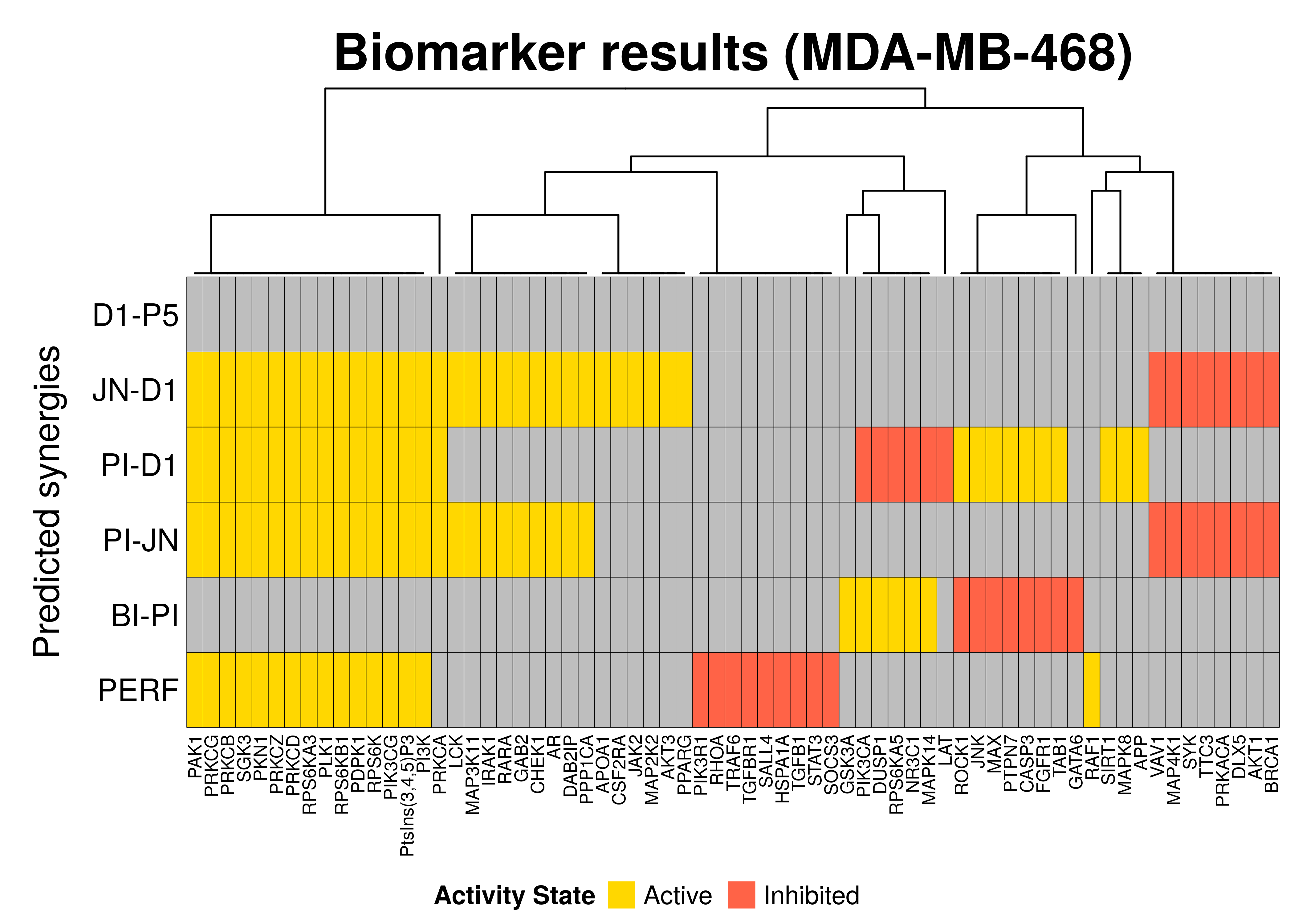
So, in general we observe that:
- A total of 67 nodes were found as biomarkers (for at least one synergy)
- Most synergies have more than 10 biomarkers. Usually we wouldn’t expect too
many biomarkers that are directly related to the prediction of a specific synergy.
The abudance of (false positive) biomarkers for some synergies (e.g.
PI-D1) relates to the model classification method used, which does not incorporate in its internal logic that the prediction of other synergies than the ones used for the grouping itself can affect the biomarker results obtained from it - We couldn’t identify any biomarkers at the \(0.7\) threshold for the
D1-P5synergy - All the active performance-related biomarkers (PERF) were also observed as
biomarkers for the prediction of a specific synergy(ies) with the exception of
the
RAF1node - There exist common biomarkers across different predicted synergies, e.g.
SGK3is a common active biomarker across 3 synergistic drug combinations - We observe that between the two predicted synergies
PI-D1andBI-PIthere are conflicted biomarkers in the sense that they have to be in an more active state for the first synergy and more inhibited for the other (and vise versa) - The synergies
JN-D1,PI-D1andPI-JNshare many common biomarkers as well as with the performance-related biomarkers