CASCADE 1.0 - Parameterization vs #fixpoints

In this section we identify the key nodes whose parameterization affects the change of dynamics of the CASCADE 1.0 network, i.e. are responsible for the change in the number of fixpoint attractors (0,1 and 2) across all link-operator mutated models.

We will use several statistical methods, in each of the sub-sections below.

The training data is a link-operator matrix, where rows are models (\(2^{23}\)), columns/features/variables are link-operator nodes (\(23\) in total) and the parameterization values correspond to \(0\) (AND-NOT) or \(1\) (OR-NOT). The ternary response for each model is a number denoting the number of fixpoints (\(0,1\) or \(2\)).

The matrix we can generate with the script get_lo_mat.R and the response is part of the previously generated data from the script count_models_ss.R.

Multinomial LASSO

Use the script param_ss_glmnet.R to fit a multinomial LASSO model for the data (Friedman, Hastie, and Tibshirani 2010). We now simply load the result object:

fit_a1 = readRDS(file = "data/fit_a1.rds")
plot(fit_a1, xvar = "dev", type.coef = "2norm")
plot(fit_a1, xvar = "lambda", type.coef = "2norm")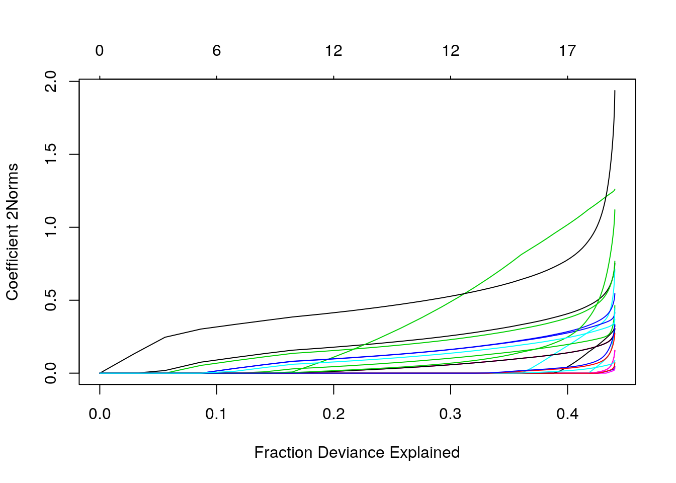

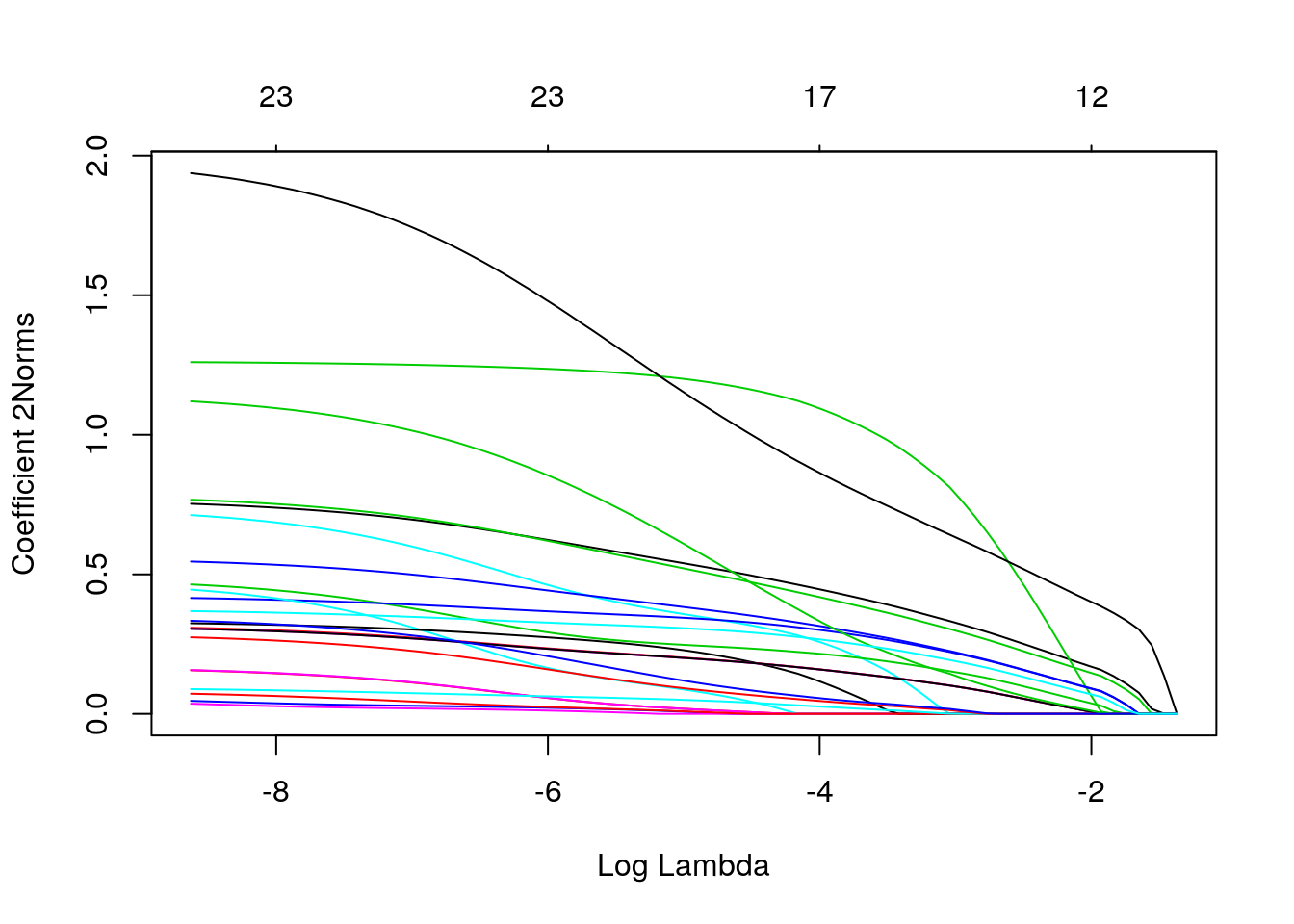
Figure 3: Euclidean Norm of glment coefficients vs lambda and deviance explained

As we can see there is no \(\lambda\) that could explain more than \(44\%\) of the deviance and there are a lot of non-zero coefficients associated with smaller values of \(\lambda\). For example, choosing \(\lambda = 0.0142\) (tested prediction accuracy \(\approx 0.72\) on a random subset of the data), we have the following coefficients, shown in a heatmap:

# choose a lambda
lambda1 = fit_a1$lambda[32]

fit_a1_coef = coef(fit_a1, s = lambda1) %>%
  lapply(as.matrix) %>%
  Reduce(cbind, x = .) %>% t()
rownames(fit_a1_coef) = names(coef(fit_a1, s = lambda1)) # 0, 1 and 2 stable states

imp_nodes_colors = rep("black", length(colnames(fit_a1_coef)))
names(imp_nodes_colors) = colnames(fit_a1_coef)
imp_nodes_colors[names(imp_nodes_colors) %in% c("MEK_f", "PTEN", "MAPK14")] = "green4"

ComplexHeatmap::Heatmap(matrix = fit_a1_coef, name = "Coef", row_title = "Number of Fixpoints", 
  row_names_side = "right", row_dend_side = "right", row_title_side = "right",
  column_title = "Glmnet Coefficient Scores (λ = 0.0142)",
  column_dend_height = unit(20, "mm"), column_names_gp = gpar(col = imp_nodes_colors))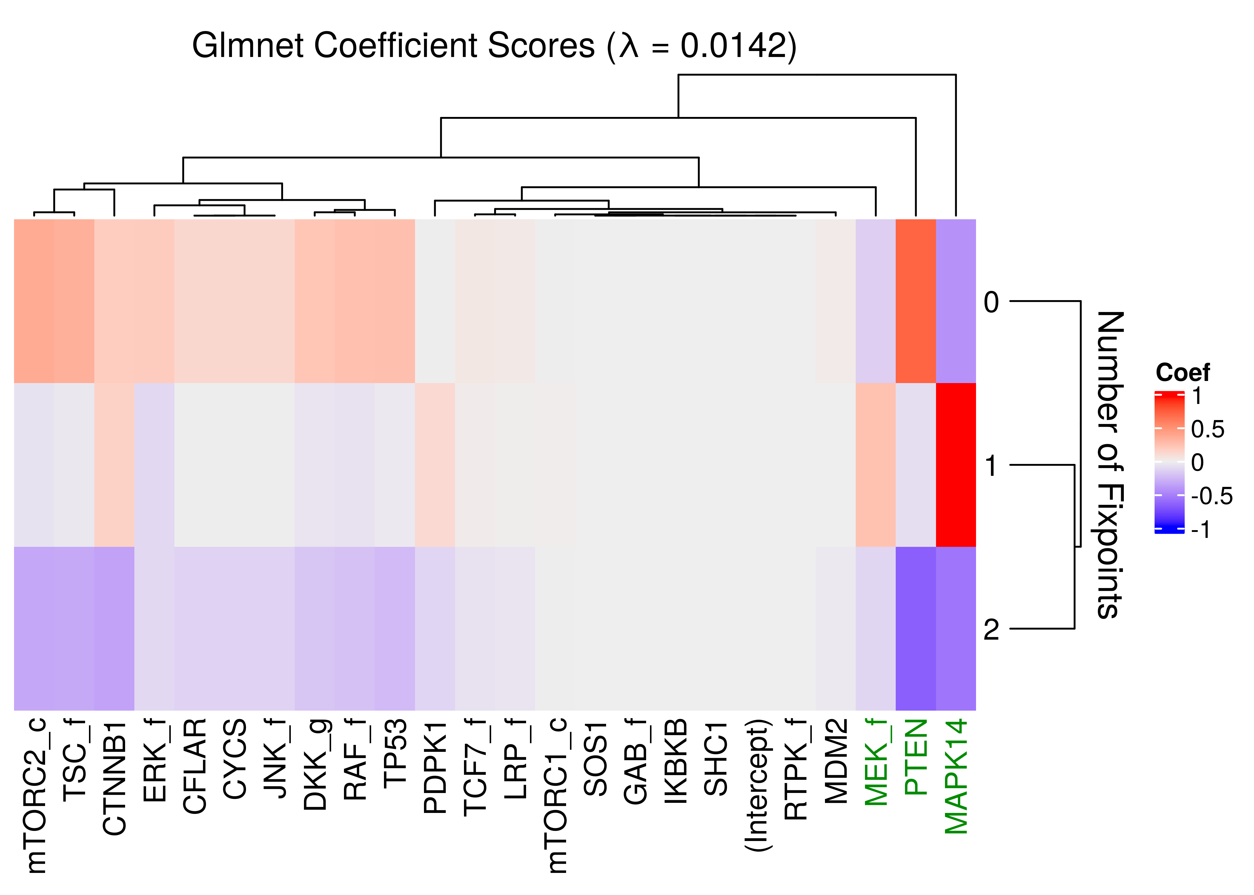

Figure 4: Heatmap of coefficients of multinomial model (glmnet)

# check accuracy
# lo_mat = readRDS(file = "data/lo_mat.rds")
# models_ss_stats = readRDS(file = "data/models_ss_stats.rds")
# ss_num = models_ss_stats %>% pull(ss_num)
# set.seed(42)
# model_indexes = sample(x = 1:nrow(lo_mat), size = 100000)
# pred = predict(object = fit_a1, newx = lo_mat[model_indexes, ],
#   type = "class", s = lambda1) %>% as.integer()
# acc = sum(pred == ss_num[model_indexes])/length(pred)
# print(acc) # should be ~ 0.72

Even thought the glmnet classifier might not be accurate enough, we still find that the nodes PTEN and MAPK14 are the most important (larger coefficients) for distinguishing between the models with different number of fixpoints. Additional nodes (like MEK_f and CTNNB1) are likely to be important as well.

If we cross-validate the regularization parameter \(\lambda\) (using the same script, we randomly selected smaller model samples - \(100000\), \(20\) times in total), and choose the \(\lambda_{1se}\) for each different run to get the coefficients, the results can be visualized as follows:

cvfit_data = readRDS(file = "data/cvfit_data.rds")
cvfit_mat_list = lapply(cvfit_data, function(cvfit) {
  co = coef(cvfit) %>% 
    lapply(as.matrix) %>%
    Reduce(cbind, x = .) %>% 
    t()
  rownames(co) = names(coef(cvfit)) # 0,1 and 2 stable states
  return(co)
})

cvfit_mat = do.call(rbind, cvfit_mat_list)

imp_nodes_colors = rep("black", length(colnames(cvfit_mat)))
names(imp_nodes_colors) = colnames(cvfit_mat)
imp_nodes_colors[names(imp_nodes_colors) %in% c("MEK_f", "PTEN", "MAPK14", "CTNNB1", "mTORC1_c")] = "green4"

ComplexHeatmap::Heatmap(matrix = cvfit_mat, name = "Coef", row_title = "Number of Fixpoints", 
  row_dend_side = "right", row_title_side = "left",
  column_title = "Glmnet Coefficient Scores", row_km = 3, row_km_repeats = 10, 
  show_row_names = FALSE, column_dend_height = unit(20, "mm"),
  column_names_gp = gpar(col = imp_nodes_colors),
  left_annotation = rowAnnotation(foo = anno_block(
    labels = c("2", "1", "0"), # with `show_row_names = TRUE` you can check this
    labels_gp = gpar(col = "black", fontsize = 12))))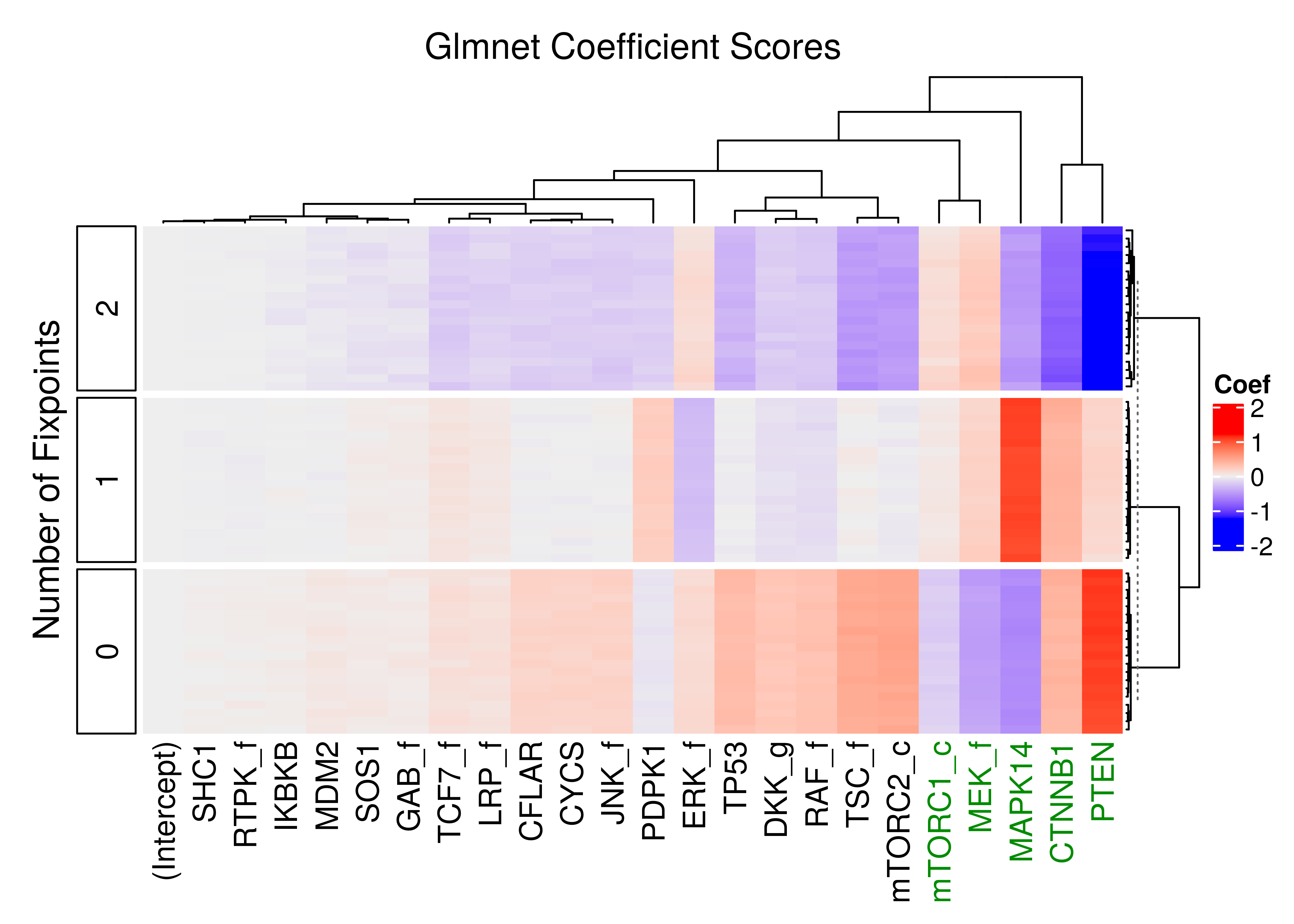

Figure 5: Heatmap of coefficients of multinomial model (glmnet - 20 CV models)

The top 5 most important nodes are seen in green in the above heatmap: MAPK14, PTEN, CTNNB1, MEK_f and mTORC1_c.

Random Forests

We used the param_ss_randf.R script to tune and train a random forest classifier on the dataset (Liaw and Wiener 2002). First we tuned the mtry parameter, the number of variables randomly selected at each tree split:

mtry_data = readRDS(file = "data/mtry_data.rds")

mtry_data %>%
  ggplot(aes(x = mtry, y = OOBError, group = mtry)) +
  geom_boxplot(fill = "green4") +
  labs(title = "Tuning Random Forest mtry parameter") +
  theme_classic(base_size = 14) + theme(plot.title = element_text(hjust = 0.5))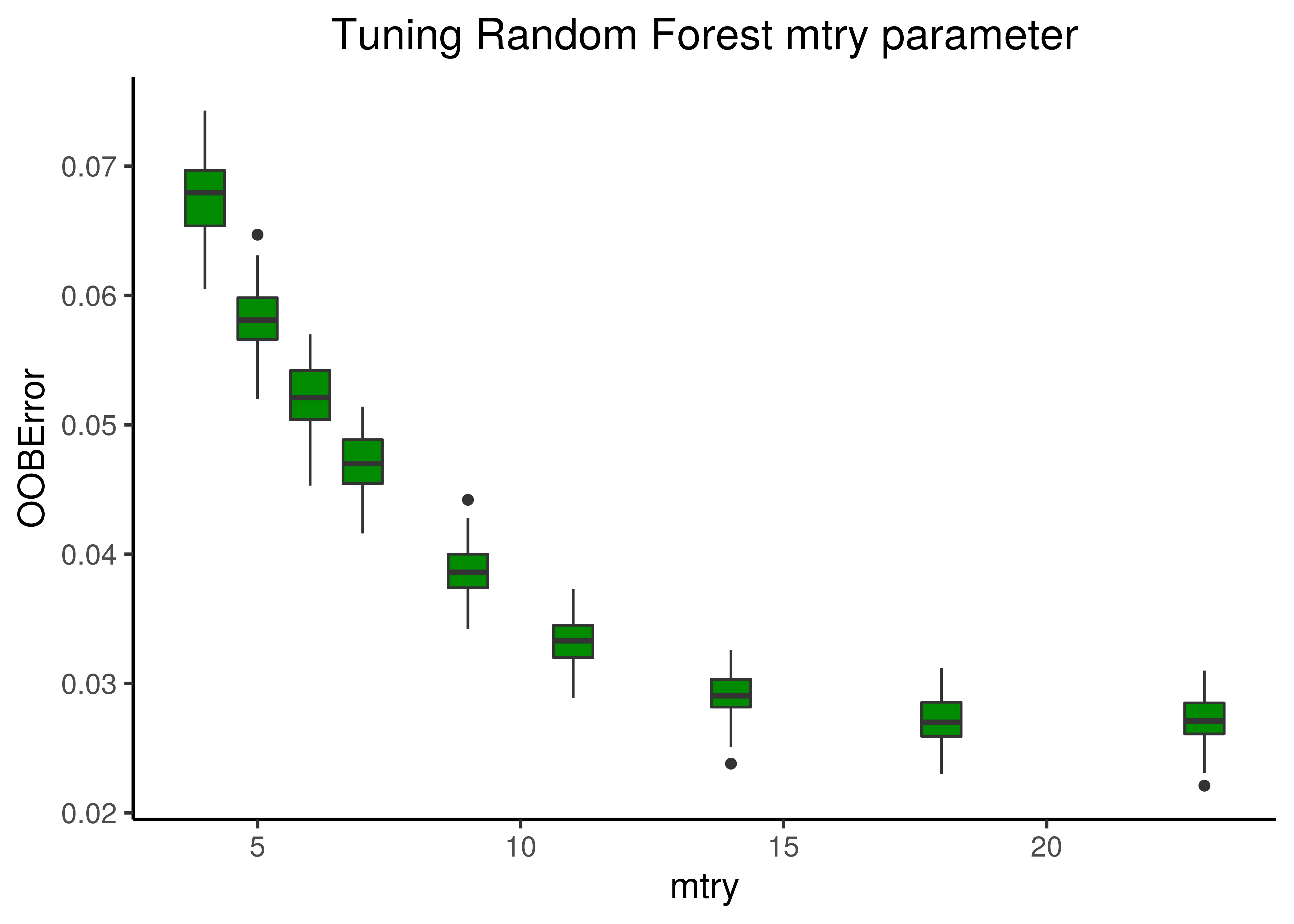

Figure 6: Random Forest Tuning (mtry)

A value between \(14-18\) for mtry seems to minimize the Out-Of-Bag Error, so we choose \(16\) for the rest of the analysis. For the number of trees parameter, we stayed with the default value (\(500\)) as we observed that they were more than enough after a few test runs.

Next, we randomly selected \(100000\) models from the dataset - a total of \(20\) times - to train the random forest classifier and find the importance score of each node. We load the result data and tidy up a bit:

rf_imp_data = readRDS(file = "data/rf_imp_data.rds")

# make a list of tibbles
tbl_list = lapply(rf_imp_data, function(mat) {
  nodes = rownames(mat)
  tibble::as_tibble(mat) %>% mutate(nodes = nodes)
})

# OneForAll
imp_res = dplyr::bind_rows(tbl_list)

# Get the importance stats
imp_stats = imp_res %>% 
  group_by(nodes) %>% 
  summarise(mean_acc  = mean(MeanDecreaseAccuracy), 
            sd_acc    = sd(MeanDecreaseAccuracy), 
            mean_gini = mean(MeanDecreaseGini), 
            sd_gini   = sd(MeanDecreaseGini), 
            .groups = 'keep') %>% 
  ungroup()

The importance scores for each node were the mean decrease in accuracy and node impurity (Gini Index). We calculate the mean importance and standard deviation scores across all random samples for both measures of importance:

# color first 5 nodes in x axis
imp_col = c(rep("green4", 5), rep("grey30", nrow(imp_stats)-5))
imp_stats %>%
  mutate(nodes = forcats::fct_reorder(nodes, desc(mean_acc))) %>%
  ggplot(aes(x = nodes, y = mean_acc, fill = mean_acc)) +
  geom_bar(stat = "identity", show.legend = FALSE) +
  scale_fill_gradient(low = "steelblue", high = "red") +
  geom_errorbar(aes(ymin=mean_acc-sd_acc, ymax=mean_acc+sd_acc), width = 0.2) +
  theme_classic(base_size = 14) + 
  theme(axis.text.x = element_text(angle = 90, colour = imp_col)) +
  labs(title = "Random Forest Variable Importance (Accuracy)", 
    x = "Nodes", y = "Mean Decrease Accuracy")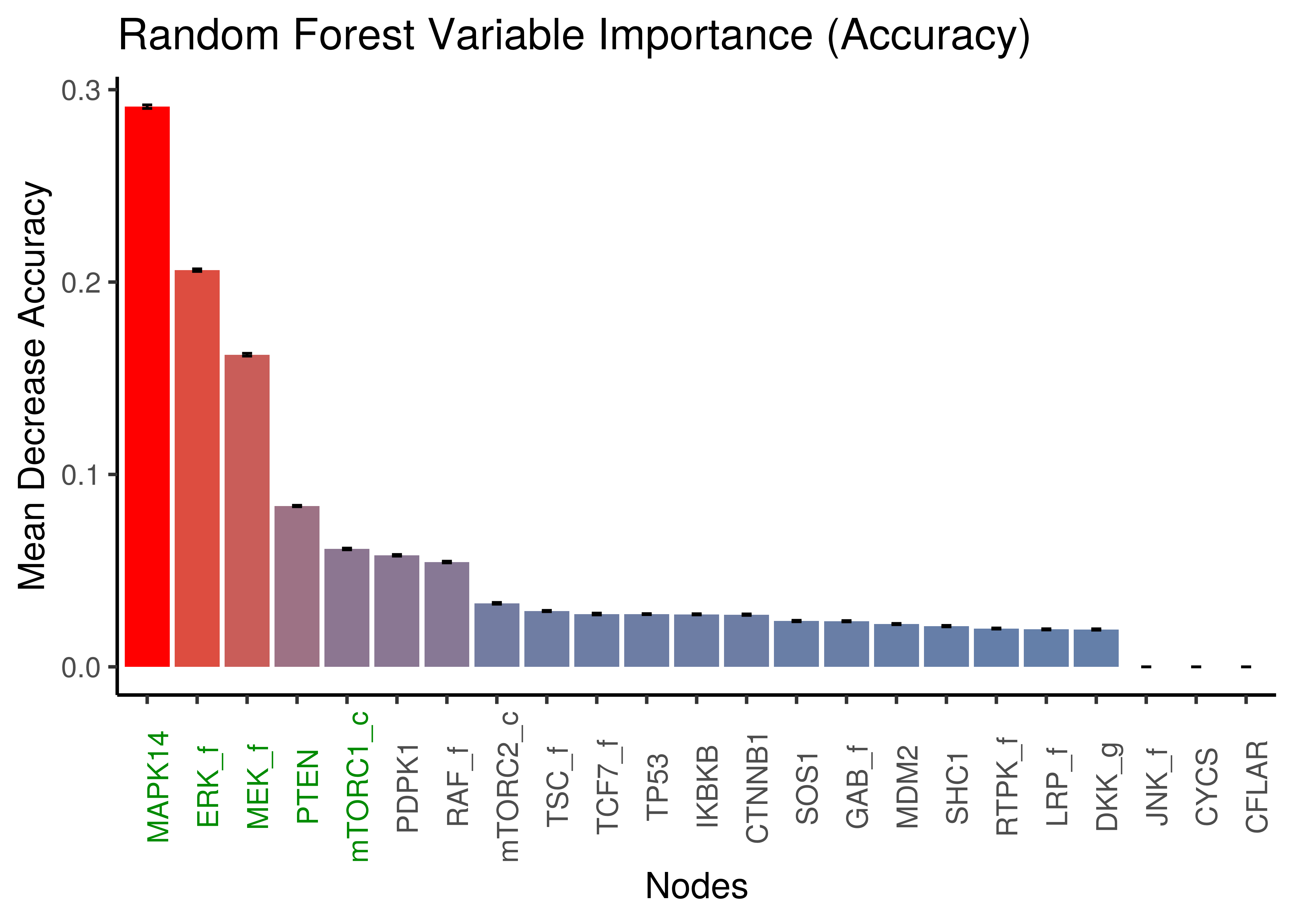

Figure 7: Random Forest: Mean Decrease Accuracy per node

imp_stats %>%
  mutate(nodes = forcats::fct_reorder(nodes, desc(mean_gini))) %>%
  ggplot(aes(x = nodes, y = mean_gini, fill = mean_gini)) +
  geom_bar(stat = "identity", show.legend = FALSE) +
  scale_fill_gradient(low = "steelblue", high = "red") +
  geom_errorbar(aes(ymin = mean_gini-sd_gini, ymax = mean_gini+sd_gini), width = 0.2) +
  theme_classic(base_size = 14) + 
  theme(axis.text.x = element_text(angle = 90, colour = imp_col)) +
  labs(title = "Random Forest Variable Importance (Gini Index)", 
    x = "Nodes", y = "Mean Decrease in Node Impurity")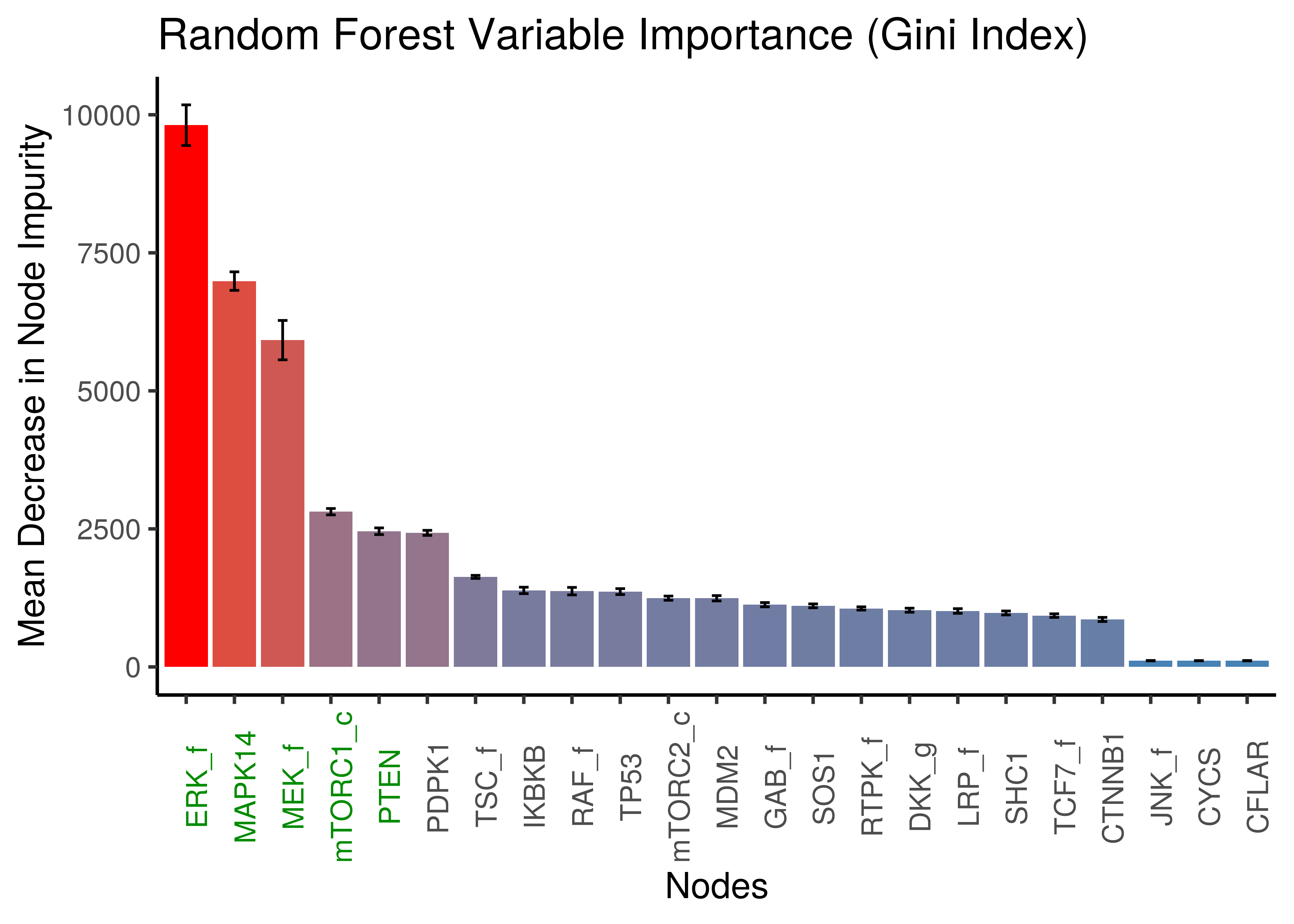

Figure 8: Random Forest: Mean Decrease in Node Impurity (Gini Index)

The top 5 important nodes by any of the two importance measures using random forests, include the nodes found as important with the LASSO method: MAPK14, ERK_f, MEK_f, PTEN, mTORC1_c.

Same results we get when using a faster, more memory efficient and with multi-thread support, random forest R package, namely ranger (Wright and Ziegler 2017). Use the script param_ss_ranger.R to reproduce the results:

ranger_res = readRDS(file = "data/ranger_res.rds")
imp_res = tibble(nodes = names(ranger_res$variable.importance), 
  gini_index = ranger_res$variable.importance)

imp_res %>% 
  mutate(nodes = forcats::fct_reorder(nodes, desc(gini_index))) %>%
  ggplot(aes(x = nodes, y = gini_index, fill = gini_index)) +
    geom_bar(stat = "identity", show.legend = FALSE) +
    scale_fill_gradient(low = "steelblue", high = "red") +
    scale_y_continuous(labels = scales::label_number_si()) +
    theme_classic(base_size = 14) + 
    theme(axis.text.x = element_text(angle = 90, colour = imp_col)) +
    labs(title = "Random Forest (Ranger) Variable Importance (Gini Index)", 
      x = "Nodes", y = "Mean Decrease in Node Impurity")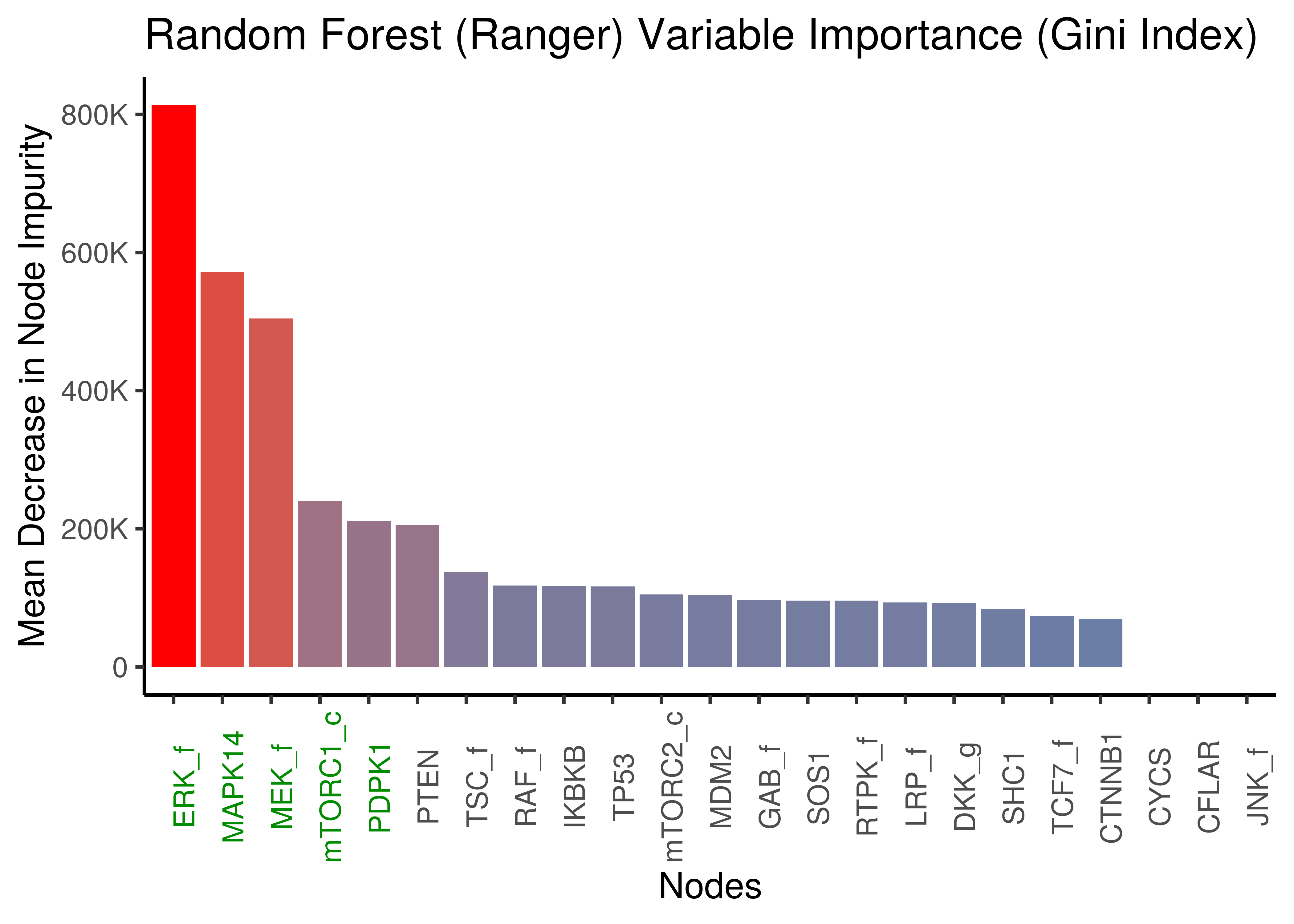

Figure 9: Random Forest (ranger): Mean Decrease in Node Impurity (Gini Index)

Parameterization Maps

We use UMAP (McInnes, Healy, and Melville 2018) to reduce the dimension of our dataset from \(23\) (number of nodes with link operators) to \(2\) and visualize it, to see if there is any apparent visual relation between the model parameterization and number of fixpoints.

We used the param_ss_umap.R script to run the UMAP implementation offered by the uwot R package. We tried various values for the n_neighbors parameter where larger values result in more global views of the dataset, while smaller values result in more local data being preserved. Also, the distance metric between the model parameterization vectors was mostly set to the standard (euclidean), but we also tried the hamming distance which seemed appropriate because of the binary nature of the dataset.

We make the figures afterwards using the result UMAP data with the param_ss_umap_vis.R script. See all the produced figures here.

Unsupervised UMAP

First we used UMAP in unsupervised mode (no a priori knowledge of the number of fixpoints per model provided or of any other information/label per model for that matter). So, UMAP is given all binary numbers from \(0\) (\(23\) \(0\)’s) to \(2^{23}-1\) (\(23\) \(1\)’s) representing each possible link operator mutated model (\(0\)’s map to AND-NOT, \(1\)’s to OR-NOT) and places them in the 2D plane.

The following figures show us the 2D parameterization map of all CASCADE 1.0 models, colored either by their decimal (base-10) number (converted from the binary link-operator model representation) or by their respective number of fixpoints:

knitr::include_graphics(path = "img/all_models_maps/umap_20nn_model_num.png")
knitr::include_graphics(path = "img/all_models_maps/umap_20nn.png")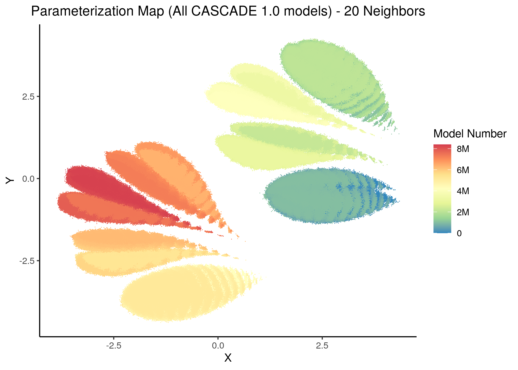

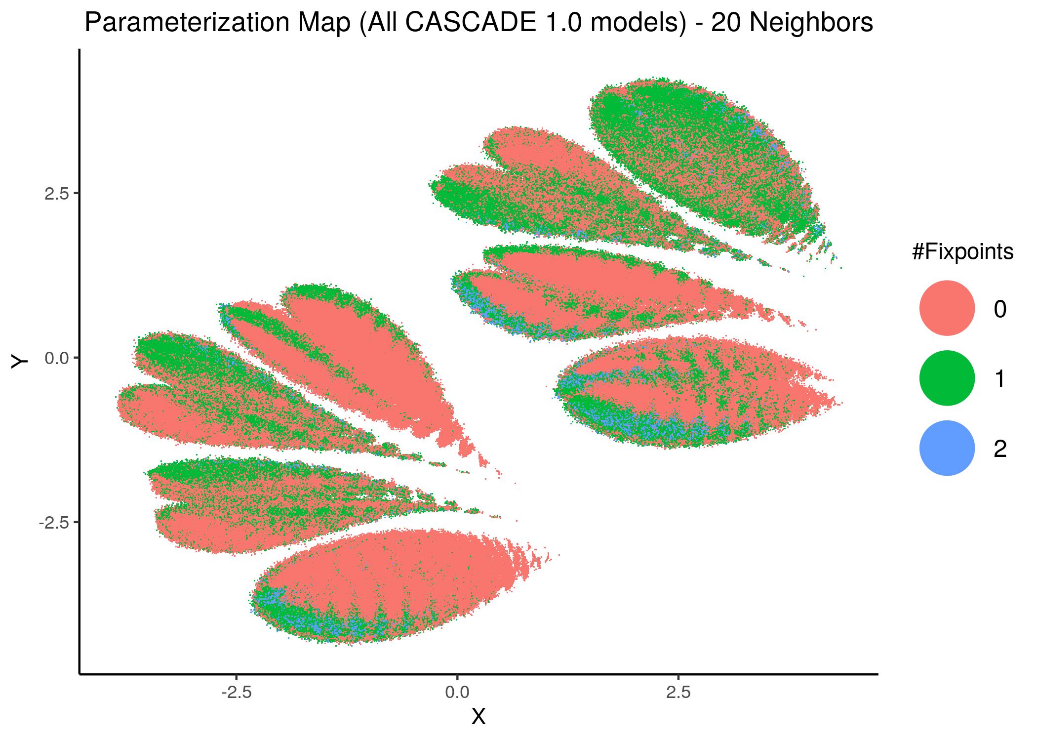
Figure 10: CASCADE 1.0 Model Parameterization Maps (euclidean distance)

knitr::include_graphics(path = "img/all_models_maps/ham_umap_20nn_model_num.png")
knitr::include_graphics(path = "img/all_models_maps/ham_umap_20nn.png")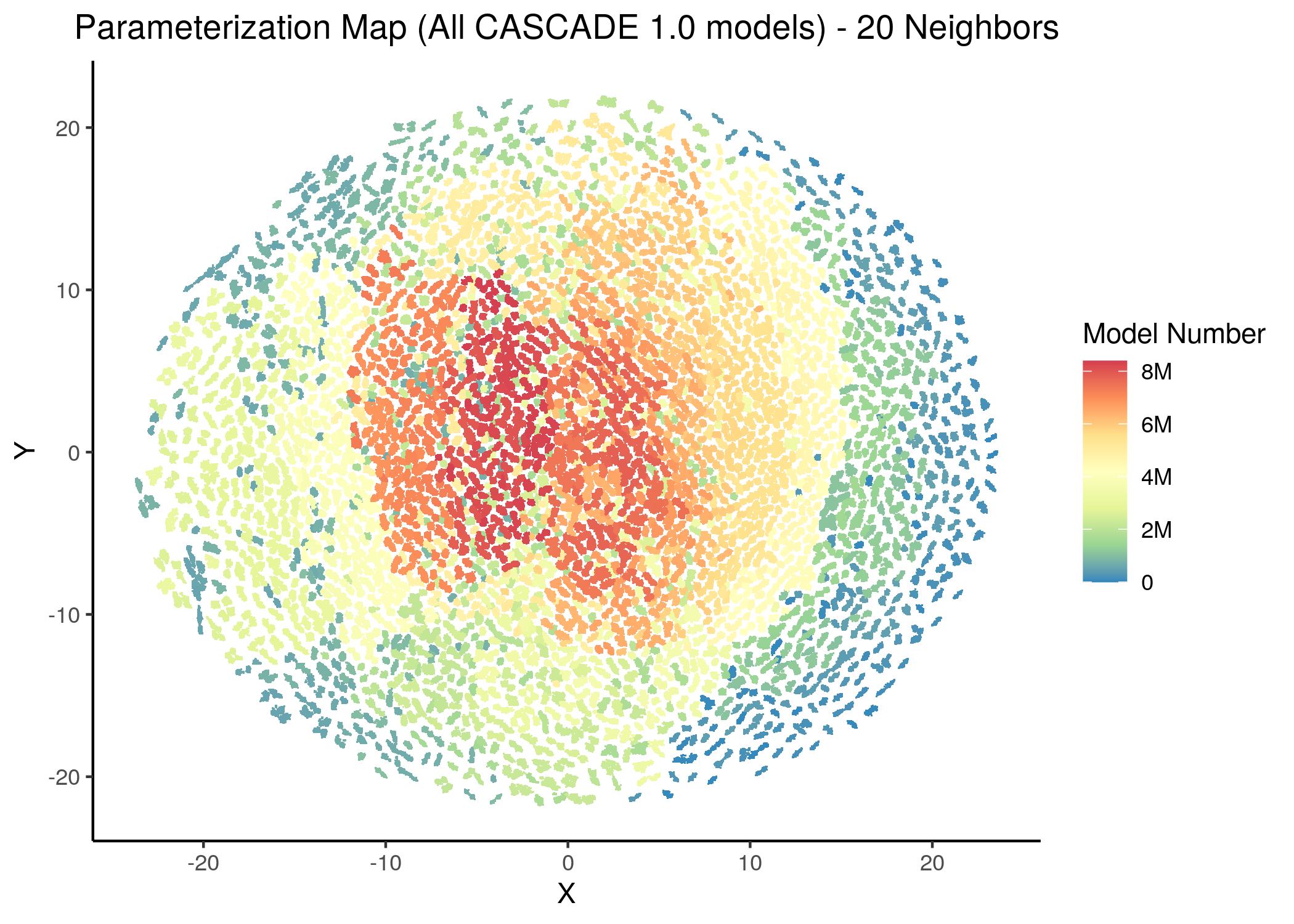

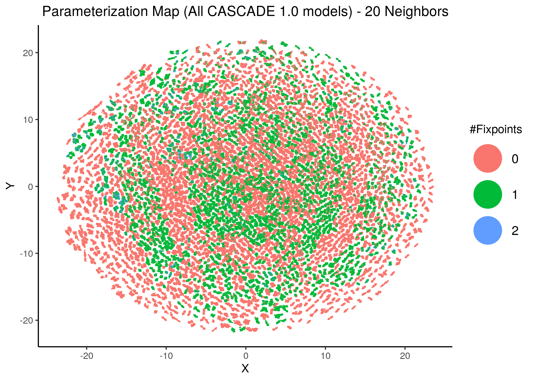
Figure 11: CASCADE 1.0 Model Parameterization Maps (hamming distance)

• Using the hamming distance metric the visualization of the dataset results in many more smaller clusters compared to the euclidean representation, which results in \(8\) neighborhoods/superclusters of similarly parameterized models. These seem to follow the numerical representation (i.e. models with close decimal numbering seem to be clustered together).
• Models with similar parameterization seem to also have the same number of fixpoints (i.e. there is some order in the placement of models that belong to the same fixpoint class - this phenomenon does not manifest chaotically - e.g. models in the same sub-cluster in the hamming parameterization map tend to have the same number of fixpoints).
• There is no distinct pattern that can match model parameterization with number of attractors. In other words, models with different number of fixpoints can manifest in no particular order whatsoever across the parameterization map/space.

Supervised UMAP

Next, we used UMAP in supervised mode - i.e. the association between each model and the corresponding fixpoint group was given as input to UMAP:

knitr::include_graphics(path = "img/all_models_maps/sumap_14nn_0_3_min_dist.png")
knitr::include_graphics(path = "img/all_models_maps/sumap_20nn.png")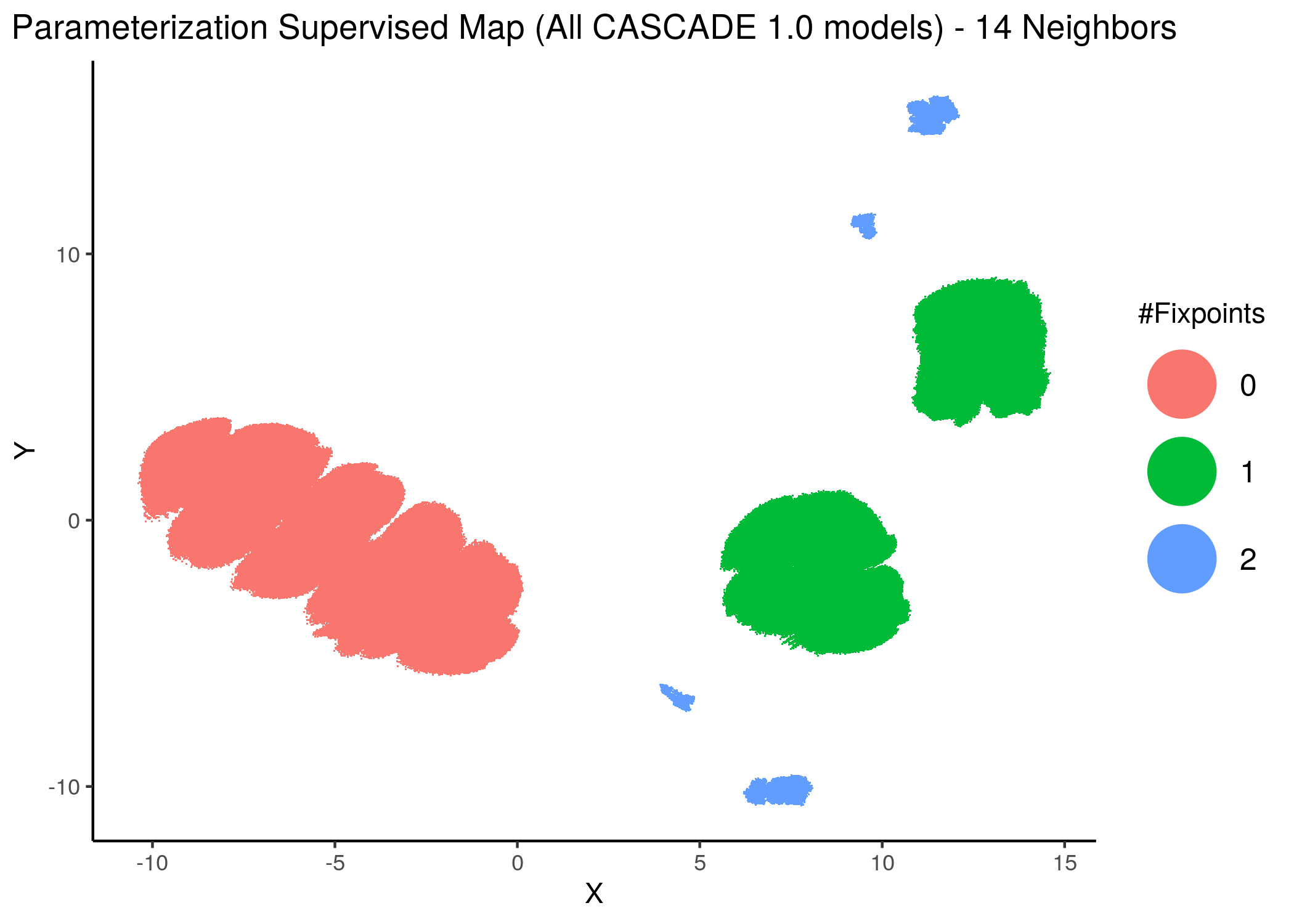

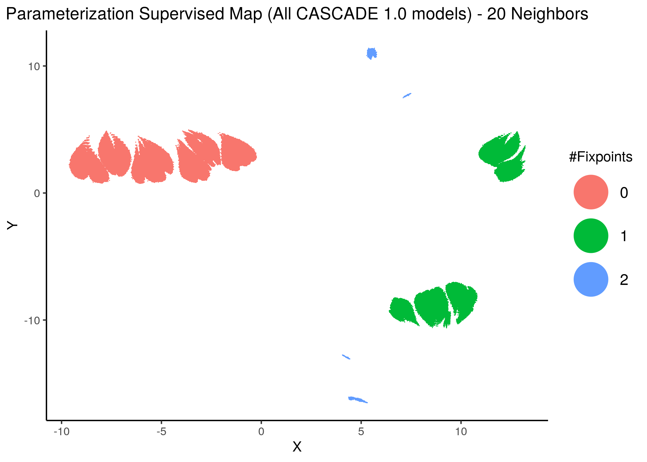
Figure 12: CASCADE 1.0 Model Parameterization Supervised Maps

With increased model complexity (meaning dynamical complexity - i.e. more attractors), the subsequent fixpoint superclusters form sub-clusters that are very differently parameterized - i.e. they form distinct families of models and thus appear to be more spread out in the supervised parameterization map.

The simple argument for this is as follows: the larger distance between a model in the \(0\) or \(1\)-fixpoint (supervised) supercluster is smaller than many of the model distances within the \(2\)-fixpoint sub-clusters.

Embedding Important Nodes in the Map

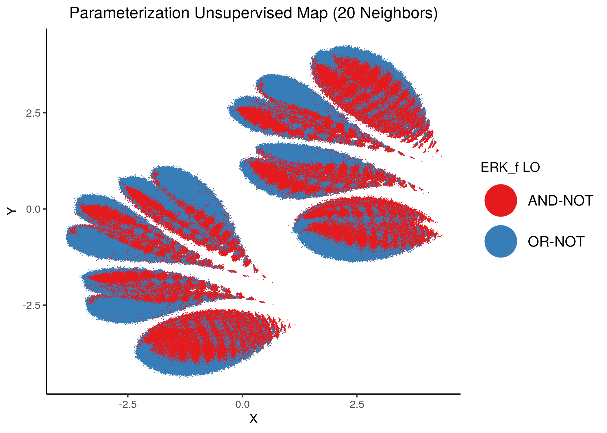
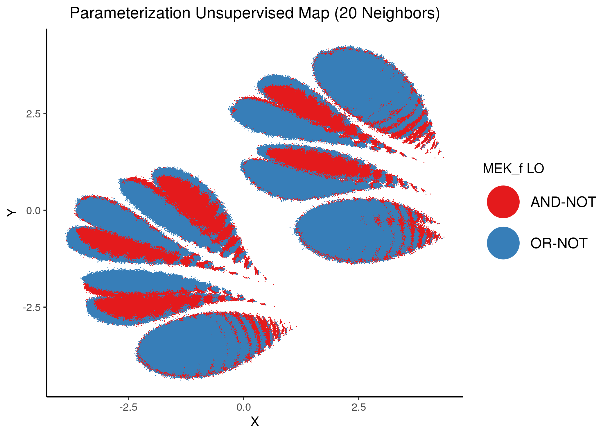
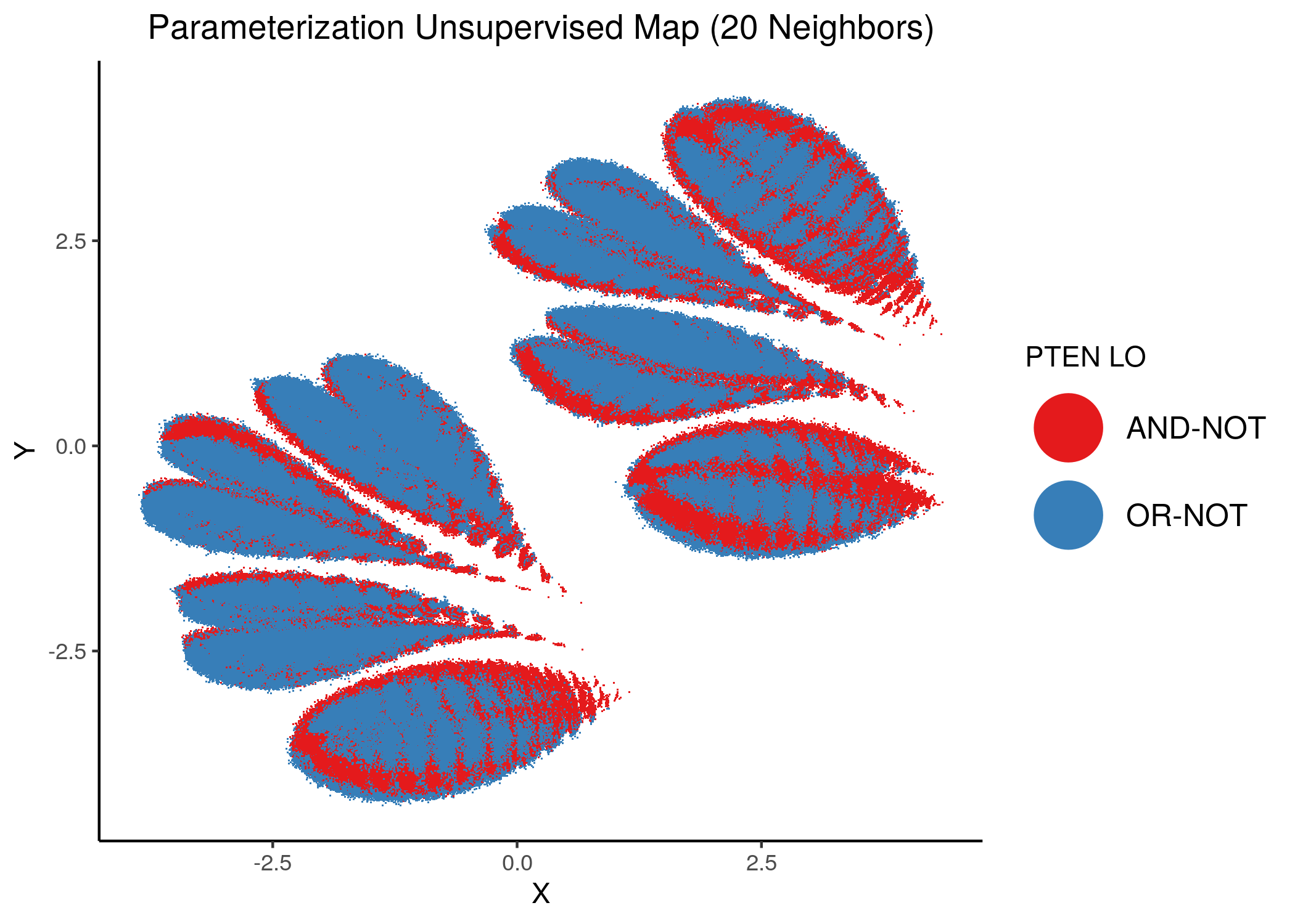
Using random forest and the regularized LASSO method, we found important nodes whose parameterization affects the change of dynamics (number of fixpoints) in the CASCADE 1.0 signaling network. Using UMAP we observed that closely parameterized models form clusters.

We will now color the UMAP parameterization maps according to the link-operator values of the top \(5\) most important nodes found from the aforementioned methods as well as the \(2\) least important node reported with random forests (use the param_ss_umap_imp_nodes.R script and see all the produced figures here).

The 3 most important nodes:

knitr::include_graphics(path = "img/imp_nodes_param_ss_maps/unsup_MAPK14.png")
knitr::include_graphics(path = "img/imp_nodes_param_ss_maps/unsup_ERK_f.png")
knitr::include_graphics(path = "img/imp_nodes_param_ss_maps/unsup_MEK_f.png")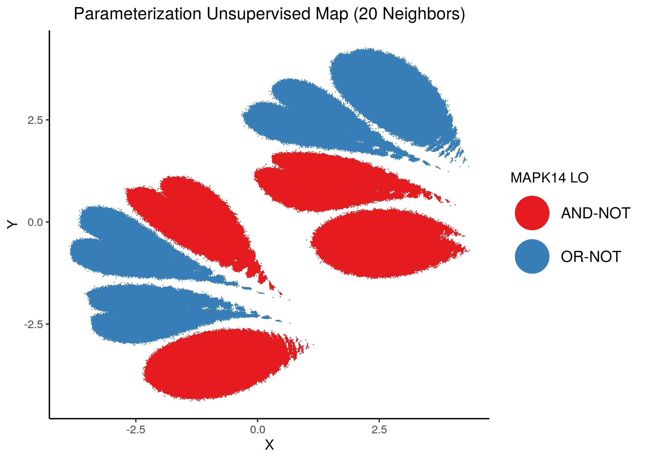

The next 2 most important nodes:

knitr::include_graphics(path = "img/imp_nodes_param_ss_maps/unsup_mTORC1_c.png")
knitr::include_graphics(path = "img/imp_nodes_param_ss_maps/unsup_PTEN.png")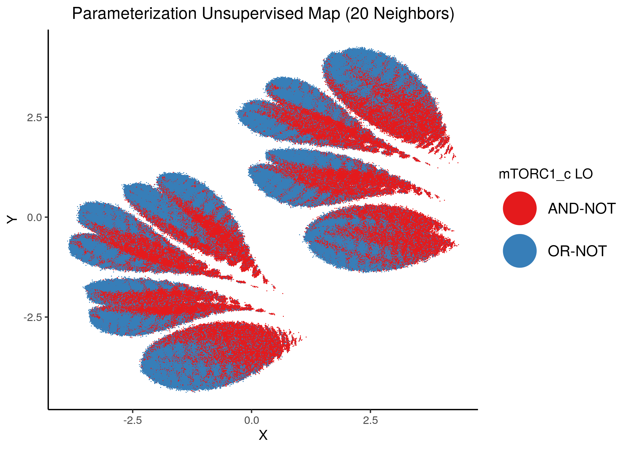

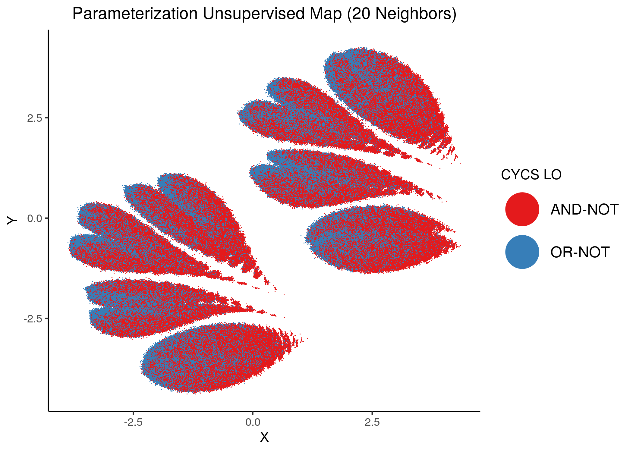
CFLAR and CYCS were the least important node for assessing the number of fixpoints of a model from its parameterization:

knitr::include_graphics(path = "img/imp_nodes_param_ss_maps/unsup_CFLAR.png")
knitr::include_graphics(path = "img/imp_nodes_param_ss_maps/unsup_CYCS.png")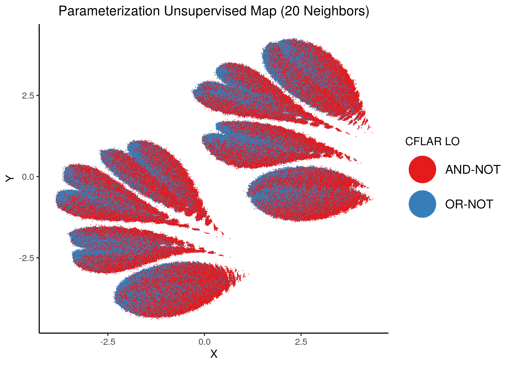

Same trend can be seen (and maybe a little more clearly) in the supervised corresponding maps:

knitr::include_graphics(path = "img/imp_nodes_param_ss_maps/sup_MAPK14.png")
knitr::include_graphics(path = "img/imp_nodes_param_ss_maps/sup_mTORC1_c.png")
knitr::include_graphics(path = "img/imp_nodes_param_ss_maps/sup_CFLAR.png")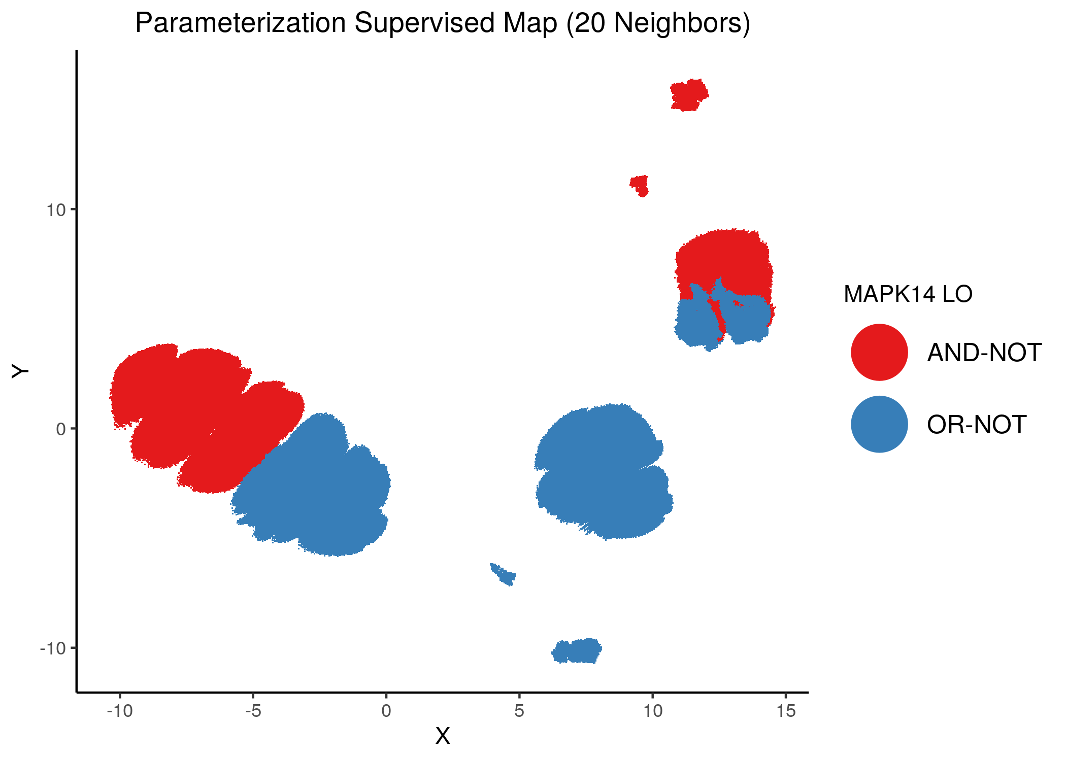

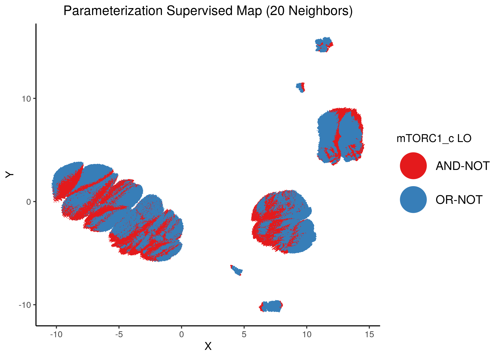
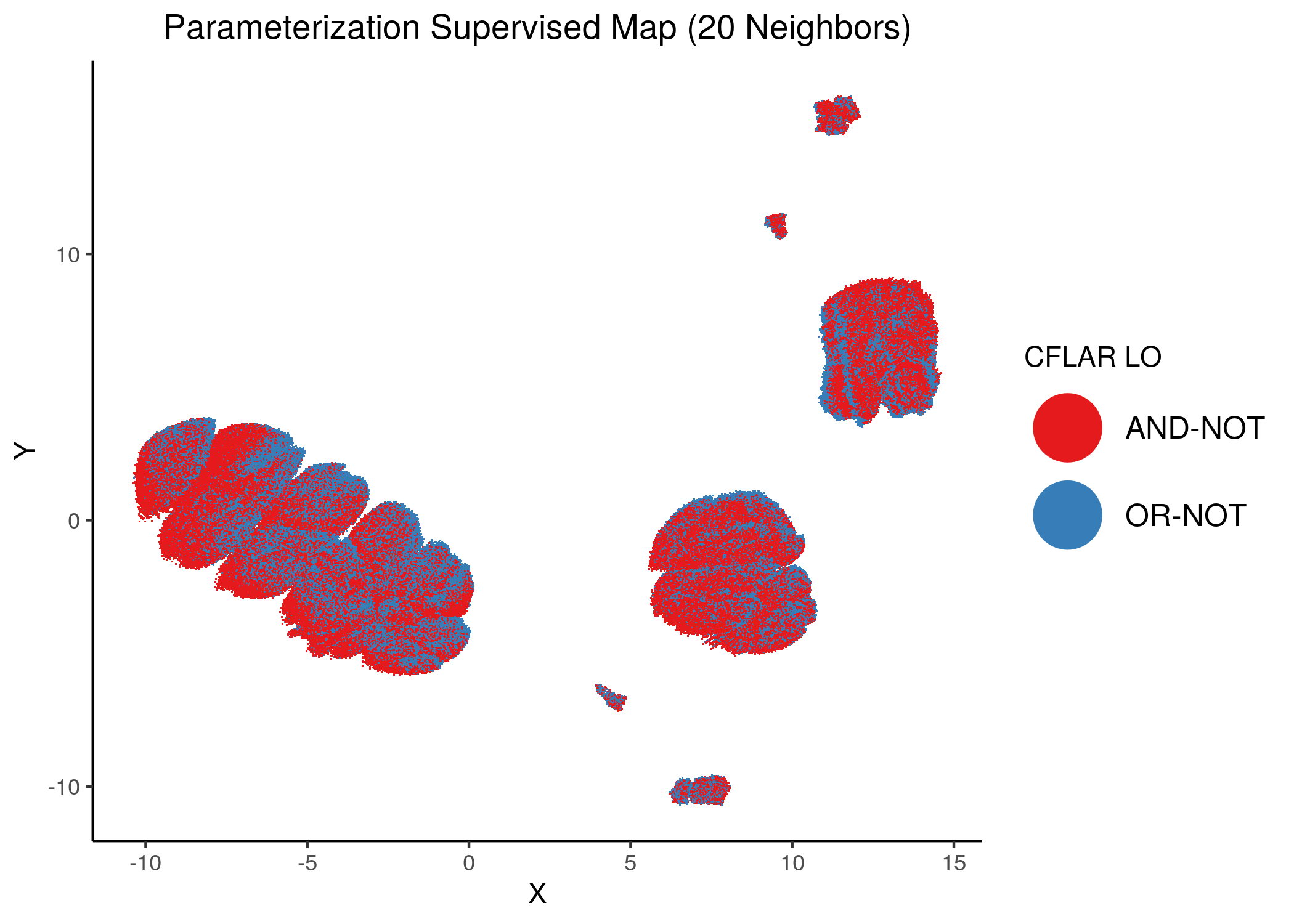
We can see a visual link between node importance (related to #fixpoints) and link operator assignment: the less important a node is, the more randomly distributed (chaotically) it’s link-operator values are across the parameterization map.

A collection of important nodes can be used to more accurately define families of closely parameterized models and as we’ve seen above this also translates to models belonging to the same fixpoint class.