Random model predictions (CASCADE 2.0) vs Number of Stable States
Last updated: 19 December, 2020
Intro
Main question: is there a relation between random models stable state number and their performance as measured by AUC PR (Precision-Recall) or AUC ROC (Receiver Operating Characteristic)?
This investigation can be considered as an extension of the random model ROC and PR curves (for CASCADE 2.0, link operator mutations) I created for the AGS paper (see version tagged v1.0 which included the abmlog-generated random model analysis here).
In that analysis, I generated a \(3000\) random model sample, and took only the models that had 1 stable state to compute their ROC performance.
So maybe I needed to generate more models or bootstrap (re-sample) these models to get a better picture of what is going on and that’s what I am trying to do here :)
Input
The random link-operator mutated models were generated from the CASCADE 2.0 topology, using the abmlog software, version 1.6.0.
Their prediction performance was assessed by the Drabme software module, via the druglogics-synergy Java module, version 1.2.0.
I run the following command to get the random models from the abmlog repo root (took ~165 min to generate all \(50000\) models):
java -cp target/abmlog-1.6.0-jar-with-dependencies.jar eu.druglogics.abmlog.RandomBooleanModelGenerator --file=test/cascade_2_0.sif --num=50000I splitted the models to 3 groups: those that have no 1 stable state, 2 stable states or none at all.
There was only 1 model in \(50000\) (cascade_2_0_418669279901714.gitsbe) that had 3 stable states and so we will not take into account models with more than 2 stable states (very rare and almost impossible to be chosen via Gitsbe since it indirectly penalizes models with more than 1 attractors).
The distribution of models in each category were (use the count_ss.sh script):
| #Stable states | #Models | Percentage |
|---|---|---|
| 0 | 29027 | 58% |
| 1 | 20672 | 41% |
| 2 | 300 | 1% |
| 3 | 1 | less than 0.01% |
From the ags_cascade_2.0 directory of the druglogics-synergy module I ran the run.sh script.
This script bootstraps \(50\) models (\(20\) times in total) from each category and runs the Drabme with those.
So bootstrapping \(50\) models \(\times \text{ }20\) times with 0 stable states, \(50\) models \(\times \text{ }20\) times with 1 stable state, etc.
We also try all pair-wise combinations: {(\(25\) models with 0 stable states) + (\(25\) models with 1 stable state)} \(\times\text{ }20\) times, etc.
Lastly, we merge all of the different stable state models together in a pool of \(25\times3=75\) models (again bootstrapping \(20\) such samples).
The generated random models and the results of the Drabme simulations are stored in
![]()
Libraries
Analysis
Note that data_dir in the next code-block is the directory where you uncompress the Zenodo dataset file (tar -xzvf boot_random_ss.tar.gz).
The ss_class denotes the model group.
E.g. ss0 is the group with models with zero stable state, ss12 is the group with half the models having 1 stable state and half of the others having 2 stable states, etc.
observed_synergies_file = "data/observed_synergies_cascade_2.0"
observed_synergies = emba::get_observed_synergies(observed_synergies_file)

data_dir = "/home/john/tmp/ags_paper_res/link-only/hsa/bootstrap_random_ss"
res_dirs = list.files(data_dir, full.names = TRUE)

data_list = list()
index = 1
for (dir in res_dirs) {
  if (stringr::str_detect(string = dir, pattern = "cascade_2.0_random_hsa_ss")) {
    # How many stable states the models had?
    ss_class = str_match(string = dir, pattern = "_(ss\\d+)_")[1,2]

    # Get the ensemble-wise synergies
    ew_syn_file = list.files(path = dir, pattern = "_ensemblewise_synergies.tab", full.names = TRUE)
    ew_synergies = emba::get_synergy_scores(ew_syn_file)

    observed = sapply(ew_synergies$perturbation %in% observed_synergies, as.integer)

    # ROC AUC (Ensemble-wise)
    ew_roc = roc.curve(scores.class0 = ew_synergies %>% pull(score) %>% (function(x) {-x}),
      weights.class0 = observed)
    ew_roc_auc = ew_roc$auc

    # PR AUC (Ensemble-wise)
    ew_pr = pr.curve(scores.class0 = ew_synergies %>% pull(score) %>% (function(x) {-x}),
  weights.class0 = observed)
    ew_pr_auc = ew_pr$auc.davis.goadrich

    # Get the model-wise synergies
    mw_syn_file = list.files(path = dir, pattern = "_modelwise_synergies.tab", full.names = TRUE)
    mw_synergies = emba::get_synergy_scores(mw_syn_file, file_type = "modelwise")

    mw_synergies = mw_synergies %>%
      mutate(synergy_prob = case_when(
        synergies == 0 & `non-synergies` == 0 ~ 0,
        TRUE ~ synergies/(synergies + `non-synergies`)))

    # ROC AUC (Model-wise)
    mw_roc = roc.curve(scores.class0 = mw_synergies %>% pull(synergy_prob), weights.class0 = observed)
    mw_roc_auc = mw_roc$auc

    # PR AUC (Model-wise)
    mw_pr = pr.curve(scores.class0 = mw_synergies %>% pull(synergy_prob), weights.class0 = observed)
    mw_pr_auc = mw_pr$auc.davis.goadrich

    # Merge results
    data_list[[index]] = dplyr::bind_cols(ss_class = ss_class,
      roc_auc = ew_roc_auc, pr_auc = ew_pr_auc, method = "ensemble-wise")
    index = index + 1
    data_list[[index]] = dplyr::bind_cols(ss_class = ss_class,
      roc_auc = mw_roc_auc, pr_auc = mw_pr_auc, method = "model-wise")
    index = index + 1
  }
}

res = dplyr::bind_rows(data_list)

saveRDS(res, file = "data/res.rds")
We will just load the result for efficiency:
Ensemble-wise Synergies
my_comparisons = list(c("ss0", "ss1"), c("ss0", "ss2"), c("ss1", "ss2"),
  c("ss0", "ss01"), c("ss1", "ss01"), c("ss2", "ss02"), c("ss01", "ss012"),  c("ss12", "ss012"))
ggboxplot(data = res %>% filter(method == "ensemble-wise"),
  x = "ss_class", y = "roc_auc", fill = "ss_class",
  xlab = "Random Model Group (#Stable States)", ylab = "ROC AUC",
  order = c("ss0", "ss1", "ss2", "ss01", "ss02", "ss12", "ss012")) +
  stat_compare_means(comparisons = my_comparisons, method = "wilcox.test", label = "p.signif")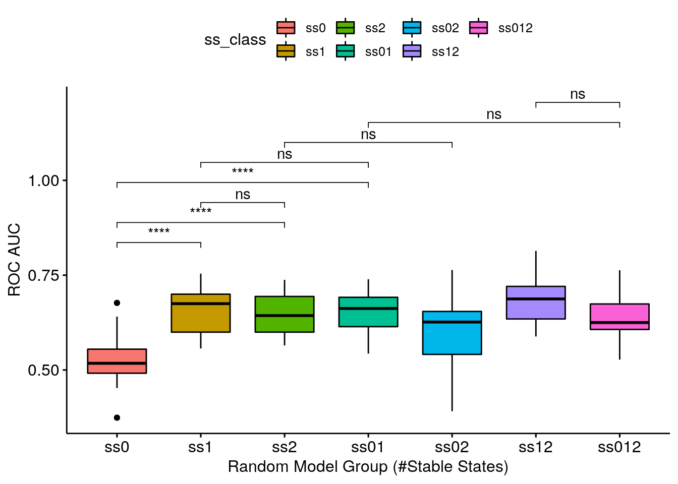
ggboxplot(data = res %>% filter(method == "ensemble-wise"),
  x = "ss_class", y = "pr_auc", fill = "ss_class",
  xlab = "Random Model Group (#Stable States)", ylab = "PR AUC",
  order = c("ss0", "ss1", "ss2", "ss01", "ss02", "ss12", "ss012")) +
  stat_compare_means(comparisons = my_comparisons, method = "wilcox.test", label = "p.signif")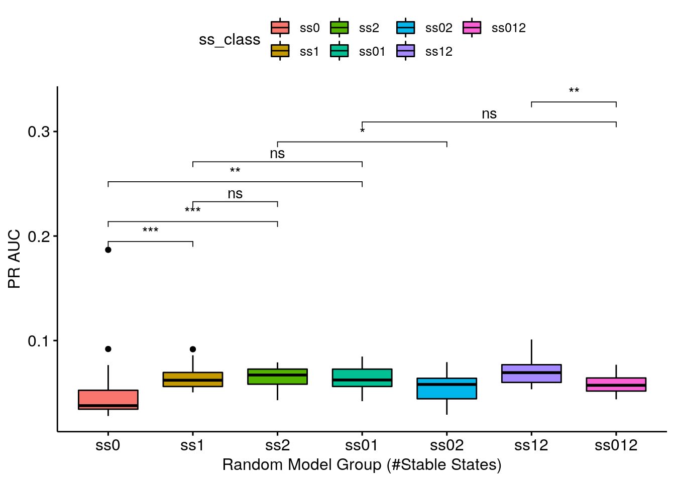
- ROC AUC results are somewhat analogous to the PR AUC results
- Getting a complete random sample of models with 1 stable state is enough to give you a valid ROC AUC (average AUC: 0.659212) - the ss1 group is one of the highest-performing groups
- Getting a decent random sample (keeping true to the models proportions as seeing in the table above) means being close to what the class ss01 represents. The class ss01 is 50-50 and a genuine decent random sample would be ~60-40 (60% models with 0 stable states and 40% models with 1 stable state), but we see that the 0 stable state models do not add AUC points (if I am allowed such terminology :) to any group that they are combined with!
- Continuing, the ss01 group is indistiguisable performance-wise from the ss1 group - meaning that using just the \(1\) stable state models as a random sample for this topology (CASCADE 2.0) is a good enough choice!
Model-wise Synergies
ggboxplot(data = res %>% filter(method == "model-wise"),
  x = "ss_class", y = "roc_auc", fill = "ss_class",
  xlab = "Random Model Group (#Stable States)", ylab = "ROC AUC",
  order = c("ss0", "ss1", "ss2", "ss01", "ss02", "ss12", "ss012")) +
  stat_compare_means(comparisons = my_comparisons, method = "wilcox.test", label = "p.signif")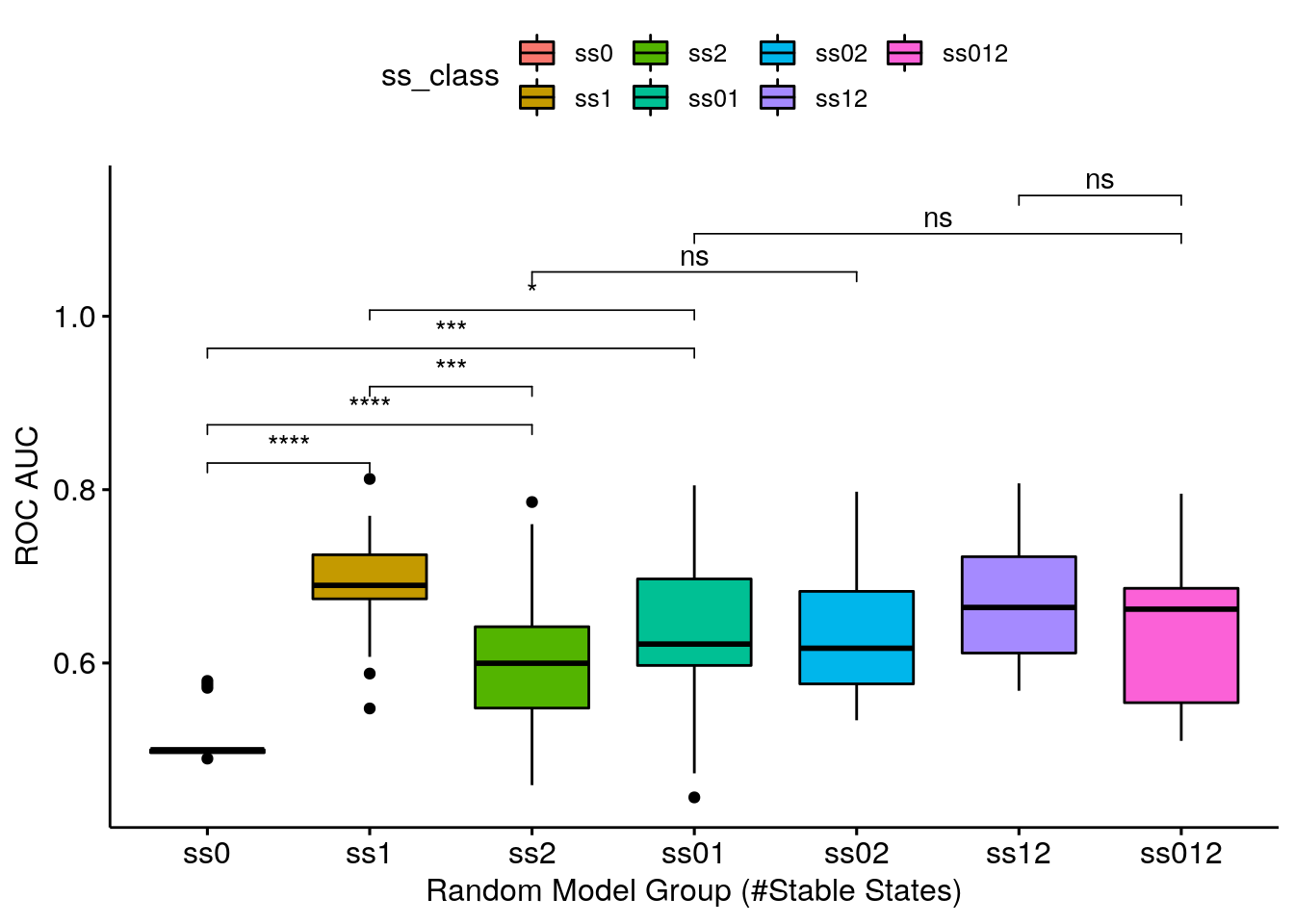
ggboxplot(data = res %>% filter(method == "model-wise"),
  x = "ss_class", y = "pr_auc", fill = "ss_class",
  xlab = "Random Model Group (#Stable States)", ylab = "PR AUC",
  order = c("ss0", "ss1", "ss2", "ss01", "ss02", "ss12", "ss012")) +
  stat_compare_means(comparisons = my_comparisons, method = "wilcox.test", label = "p.signif")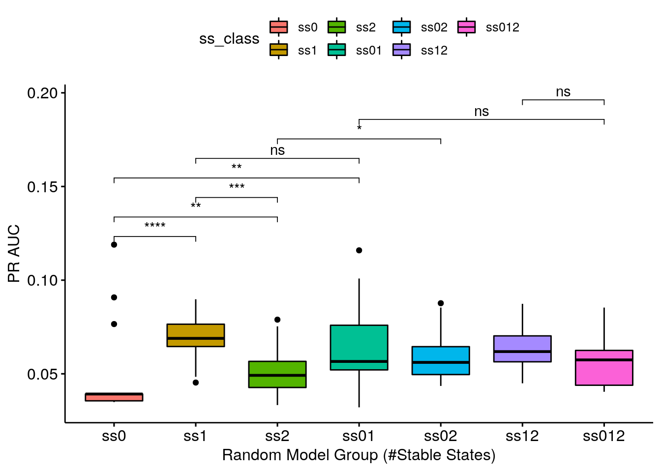
- Same results as above. Note that the model-wise methodology (used to calculate the synergy scores) seems to be more granular: it’s easier to distinguish the different categories performance using this methodology.
R session info
R version 3.6.3 (2020-02-29)
Platform: x86_64-pc-linux-gnu (64-bit)
Running under: Ubuntu 20.04.1 LTS

Locale:
  LC_CTYPE=en_US.UTF-8       LC_NUMERIC=C
  LC_TIME=en_US.UTF-8        LC_COLLATE=en_US.UTF-8
  LC_MONETARY=en_US.UTF-8    LC_MESSAGES=en_US.UTF-8
  LC_PAPER=en_US.UTF-8       LC_NAME=C
  LC_ADDRESS=C               LC_TELEPHONE=C
  LC_MEASUREMENT=en_US.UTF-8 LC_IDENTIFICATION=C

Package version:
  abind_1.4-5              assertthat_0.2.1         backports_1.2.1
  base64enc_0.1.3          BH_1.72.0.3              bookdown_0.21
  boot_1.3.25              brio_1.1.0               broom_0.7.3
  callr_3.5.1              car_3.0-10               carData_3.0-4
  cellranger_1.1.0         Ckmeans.1d.dp_4.3.3      cli_2.2.0
  clipr_0.7.1              colorspace_2.0-0         compiler_3.6.3
  conquer_1.0.2            corrplot_0.84            cowplot_1.1.0
  cpp11_0.2.4              crayon_1.3.4             curl_4.3
  data.table_1.13.4        desc_1.2.0               diffobj_0.3.2
  digest_0.6.27            dplyr_1.0.2              ellipsis_0.3.1
  emba_0.1.8               evaluate_0.14            fansi_0.4.1
  farver_2.0.3             forcats_0.5.0            foreign_0.8-75
  gbRd_0.4-11              generics_0.1.0           ggplot2_3.3.2
  ggpubr_0.4.0             ggrepel_0.9.0            ggsci_2.9
  ggsignif_0.6.0           glue_1.4.2               graphics_3.6.3
  grDevices_3.6.3          grid_3.6.3               gridExtra_2.3
  gtable_0.3.0             haven_2.3.1              highr_0.8
  hms_0.5.3                htmltools_0.5.0          htmlwidgets_1.5.3
  igraph_1.2.6             isoband_0.2.3            jsonlite_1.7.2
  knitr_1.30               labeling_0.4.2           lattice_0.20.41
  lifecycle_0.2.0          lme4_1.1.26              magrittr_2.0.1
  maptools_1.0.2           markdown_1.1             MASS_7.3.53
  Matrix_1.2.18            MatrixModels_0.4.1       matrixStats_0.57.0
  methods_3.6.3            mgcv_1.8.33              mime_0.9
  minqa_1.2.4              munsell_0.5.0            nlme_3.1.151
  nloptr_1.2.2.2           nnet_7.3.14              openxlsx_4.2.3
  parallel_3.6.3           pbkrtest_0.4.8.6         pillar_1.4.7
  pkgbuild_1.2.0           pkgconfig_2.0.3          pkgload_1.1.0
  polynom_1.4.0            praise_1.0.0             prettyunits_1.1.1
  processx_3.4.5           progress_1.2.2           PRROC_1.3.1
  ps_1.5.0                 purrr_0.3.4              quantreg_5.75
  R6_2.5.0                 rbibutils_2.0            RColorBrewer_1.1.2
  Rcpp_1.0.5               RcppArmadillo_0.10.1.2.0 RcppEigen_0.3.3.7.0
  Rdpack_2.1               readr_1.4.0              readxl_1.3.1
  rematch_1.0.1            rematch2_2.1.2           rio_0.5.16
  rje_1.10.16              rlang_0.4.9              rmarkdown_2.6
  rprojroot_2.0.2          rstatix_0.6.0            rstudioapi_0.13
  scales_1.1.1             sp_1.4.4                 SparseM_1.78
  splines_3.6.3            statmod_1.4.35           stats_3.6.3
  stringi_1.5.3            stringr_1.4.0            testthat_3.0.0
  tibble_3.0.4             tidyr_1.1.2              tidyselect_1.1.0
  tinytex_0.28             tools_3.6.3              usefun_0.4.8
  utf8_1.1.4               utils_3.6.3              vctrs_0.3.5
  viridisLite_0.3.0        visNetwork_2.0.9         waldo_0.2.3
  withr_2.3.0              xfun_0.19                yaml_2.2.1
  zip_2.1.1